Eureka Math Precalculus Module 3 Lesson 12 Answer Key

Engage NY Eureka Math Precalculus Module 3 Lesson 12 Answer Key

Eureka Math Precalculus Module 3 Lesson 12 Exercise Answer Key

Opening Exercise
Analyze the end behavior of each function below. Then, choose one of the functions, and explain how you determined the end behavior.
a. f(x) = x⁴
Answer:
As x → ∞, f(x) → ∞. As x → – ∞, f(x) → ∞.
We have 2⁴ = 16, and 3⁴ = 81. In general, as we use larger and larger inputs, this function produces larger and larger outputs, exceeding all bounds.
f is an even function, so the same remarks apply to negative inputs.

b. g(x) = – x⁴
Answer:
As x → ∞, g(x) → – ∞. As x → – ∞, g(x) → – ∞.
We have – 2⁴ = – 16, and – 3⁴ = – 81. In general, as we use larger and larger inputs, this function produces larger and larger negative outputs, exceeding all bounds.
g is an even function, so the same remarks apply to negative inputs.

c. h(x) = x³
Answer:
As x → ∞, h(x) → ∞. As x → – ∞, h(x) → – ∞.
We have 2³ = 8, and 3³ = 27. In general, as we use larger and larger inputs, this function produces larger and larger outputs, exceeding all bounds.
We also have ( – 2)³ = – 8, and ( – 3)³ = – 27. In general, as we use lesser and lesser inputs, this function produces larger and larger negative outputs, exceeding all bounds.

d. k(x) = – x³
Answer:
As x → ∞, k(x) → – ∞. As x → – ∞, k(x) → ∞.
We have – 2³ = – 8, and – 3³ = – 27. In general, as we use larger and larger inputs, this function produces larger and larger negative outputs, exceeding all bounds.
We also have – ( – 2)³ = 8, and – ( – 3)³ = 27. In general, as we use lesser and lesser inputs, this function produces larger and larger outputs, exceeding all bounds.

Exercises
Determine the end behavior of each rational function below.
Exercise 1.
f(x) = \(\frac{7 x^{5} – 3 x + 1}{4 x^{3} + 2}\)
Answer:
This function has the same end behavior as
\(\frac{7 x^{5}}{4 x^{3}}\) = \(\frac{7}{4}\)x²
Using this model as a guide, we conclude that f(x) → ∞ as x → ∞ and that f(x) → ∞ as x → – ∞.

Exercise 2.
f(x) = \(\frac{7 x^{3} – 3 x + 1}{4 x^{3} + 2}\)
Answer:
This function has the same end behavior as
\(\frac{7 x^{3}}{4 x^{3}}\) = \(\frac{7}{4}\)
Using this model as a guide, we conclude that f(x) → \(\frac{7}{4}\) as x → ∞ and that f(x) → \(\frac{7}{4}\) as x → – ∞.

Exercise 3.
f(x) = \(\frac{7 x^{3} + 2}{4 x^{5} – 3 x + 1}\)
Answer:
This function has the same end behavior as
\(\frac{7 x^{3}}{4 x^{5}}\) = \(\frac{7}{4 x^{2}}\)
Using this model as a guide, we conclude that f(x) → 0 as x → ∞ and that f(x) → 0 as x → – ∞.

Eureka Math Precalculus Module 3 Lesson 12 Problem Set Answer Key

Question 1.
Analyze the end behavior of both functions.
a. f(x) = x, g(x) = \(\frac{1}{x}\)
Answer:
For f(x): f(x) → ∞ as x → ∞, and f(x) → – ∞ as x → – ∞.
For g(x): g(x) → ∞ as x → 0, and g(x) → – ∞ as x → 0.

b. f(x) = x³, g(x) = \(\frac{1}{x^{3}}\)
Answer:
For f(x): f(x) → ∞ as x → ∞, and f(x) → – ∞ as x → – ∞.
For g(x): g(x) → ∞ as x → 0, and g(x) → – ∞ as x → 0.

c. f(x) = x², g(x) = \(\frac{1}{x^{2}}\)
Answer:
For f(x): f(x) → ∞ as x → ∞, and f(x) → ∞ as x → – ∞.
For g(x): g(x) → ∞ as x → 0, and g(x) → ∞ as x → 0.

d. f(x) = x⁴, g(x) = \(\frac{1}{x^{4}}\)
Answer:
For f(x): f(x) → ∞ as x → ∞, and f(x) → – ∞ as x → – ∞.
For g(x): g(x) → ∞ as x → 0, and g(x) → – ∞ as x → 0.

e. f(x) = x – 1, g(x) = \(\frac{1}{x – 1}\)
Answer:
For f(x): f(x) → ∞ as x → ∞, and f(x) → – ∞ as x → – ∞.
For g(x): g(x) → ∞ as x → 0, and g(x) → – ∞ as x → 0.

f. f(x) = x + 2, g(x) = \(\frac{1}{x + 2}\)
Answer:
For f(x): f(x) → ∞ as x → ∞, and f(x) → – ∞ as x → – ∞.
For g(x): g(x) → 0 as x → ∞, and g(x) → 0 as x → – ∞.

g. f(x) = x² – 4, g(x) = \(\frac{1}{x^{2} – 4}\)
Answer:
For f(x): f(x) → ∞ as x → ∞, and f(x) → – ∞ as x → – ∞.
For g(x): g(x) → ∞ a x → 0, and g(x) → – ∞ as x → 0.

Question 2.
For the following functions, determine the end behavior. Confirm your answer with a table of values.
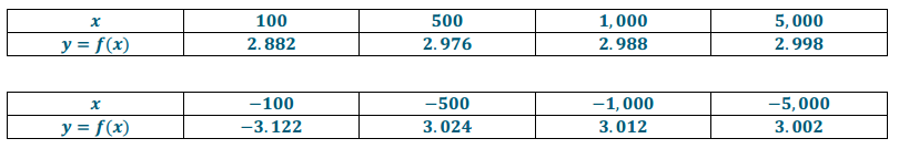
a. f(x) = \(\frac{3x – 6}{x + 2}\)
Answer:
f has the same end behavior as \(\frac{3x}{x}\) = 3. Using this model as a guide, we conclude that
f(x) → 3 as x → ∞, and f(x) → 3 as x → – ∞.

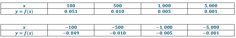
b. f(x) = \(\frac{5 x + 1}{x^{2} – x – 6}\)
Answer:
f has the same end behavior as \(\frac{5 x}{x^{2}}\) = \(\frac{5}{x}\). Using this model as a guide, we conclude that
f(x) → 0 as x → ∞, and f(x) → 0 as x → – ∞.

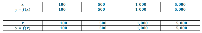
c. f(x) = \(\frac{x^{3} – 8}{x^{2} – 4}\)
Answer:
f has the same end behavior as \(\frac{x^{3}}{x^{2}}\) = x. Using this model as a guide, we conclude that
f(x) → ∞ as x → ∞, and f(x) → – ∞ as x → – ∞.

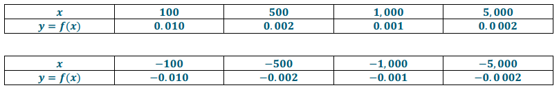
d. f(x) = \(\frac{x^{3} – 1}{x^{4} – 1}\)
Answer:
f has the same end behavior as \(\frac{x^{3}}{x^{4}}\) = \(\frac{1}{x^{\circ}}\). Using this model as a guide, we conclude that
f(x) → 0 as x → ∞, and f(x) → 0 as x → – ∞.

e. f(x) = \(\frac{(2 x + 1)^{3}}{\left(x^{2} – x\right)^{2}}\)
Answer:
f has the same end behavior as \(\frac{8 x^{3}}{x^{4}}\) = \(\frac{8}{x}\). Using this model as a guide, we conclude that
f(x) → 0 as x → ∞, and f(x) → 0 as x → – ∞.

Question 3.
For the following functions, determine the end behavior.
a. f(x) = \(\frac{5 x^{6} – 3 x^{3} + x – 2}{5 x^{4} – 3 x^{3} + x – 2}\)
Answer:
f has the same end behavior as \(\frac{5 x^{6}}{5 x^{4}}\) = x². Using this model as a guide, we conclude that
f(x) → ∞ as x → ∞, and f(x) → ∞ as x → – ∞.

b. f(x) = \(\frac{5 x^{4} – 3 x^{3} + x – 2}{5 x^{6} – 3 x^{3} + x – 2}\)
Answer:
f has the same end behavior as \(\frac{5 x^{4}}{5 x^{6}}\) = \(\frac{1}{x^{2}}\) . Using this model as a guide, we conclude that
f(x) → 0 as x → ∞, and f(x) → 0 as x → – ∞.

c. f(x) = \(\frac{5 x^{4} – 3 x^{3} + x – 2}{5 x^{4} – 3 x^{3} + x – 2}\)
Answer:
f has the same end behavior as \(\frac{5 x^{4}}{5 x^{4}}\) = 1. Using this model as a guide, we conclude that
f(x) → 1 as x → ∞, and f(x) → 1 as x → – ∞.

d. f(x) = \(\frac{\sqrt{2} x^{2} + x + 1}{3 x + 1}\)
Answer:
f has the same end behavior as \(\frac{\sqrt{2} x^{2}}{3 x}\) = \(\frac{\sqrt{2}}{3}\) x. Using this model as a guide, we conclude that
f(x) → ∞ as x → ∞, and f(x) → – ∞ as x → – ∞.

e. f(x) = \(\frac{4 x^{2} – 3 x – 7}{2 x^{3} + x – 2}\)
Answer:
f has the same end behavior as \(\frac{4 x^{2}}{2 x^{3}}\) = \(\frac{2}{x}\).
f(x) → 0 as x → ∞, and f(x) → 0 as x → – ∞.

Question 4.
Determine the end behavior of each function.
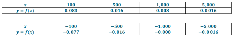
a. f(x) = \(\frac{\sin (x)}{x}\)
Answer:
– 1≤sin x≤1,
f(x) → 0 as x → ∞, and f(x) → 0 as x → – ∞.

b. f(x) = \(\frac{\cos (x)}{x}\)
Answer:
– 1≤cos x≤1,
f(x) → 0 as x → ∞, and f(x) → 0 as x → – ∞.

c. f(x) = \(\frac{2^{x}}{x}\)
Answer:
f(x) → ∞ as x → ∞, and f(x) → 0 as x → – ∞.

d. f(x) = \(\frac{x}{2^{x}}\)
Answer:
f(x) → 0 as x → ∞, and f(x) → – ∞ as x → – ∞.

e. f(x) = \(\frac{4}{1 + e^{ – x}}\)
Answer:
f(x) → 4 as x → ∞, and f(x) → 0 as x → – ∞.

f. f(x) = \(\frac{10}{1 + e^{ – x}}\)
Answer:
f(x) → 10 as x → ∞, and f(x) → 0 as x → – ∞.

Question 5.
Consider the functions f(x) = x! and g(x) = x⁵ for natural numbers x.
a. What are the values of f(x) and g(x) for x = 5, 10, 15, 20, 25?
Answer:
f(x) = {120,3 628 800,1 307 674 368 000,2.4×10¹⁸,1.6×10²⁵}
g(x) = {3125,100 000,759 375,3 200 000,9 765 625}

b. What is the end behavior of f(x) as x → ∞?
Answer:
f(x) → ∞

c. What is the end behavior of g(x) as x → ∞?
Answer:
g(x) → ∞

d. Make an argument for the end behavior of \(\) as x → ∞.
Answer:
Since y = f(x) increases so much faster than y = g(x), f(x) overpowers the division by g(x). By x = 25, \(\frac{f(x)}{g(x)}\)≈1.6×10¹⁸. Thus, \(\frac{f(x)}{g(x)}\) → ∞.

e. Make an argument for the end behavior of \(\frac{g(x)}{f(x)}\) as x → ∞.
Answer:
For the same reasons as in part (d), division by f(x) overpowers g(x) in the numerator. By x = 25, \(\frac{g(x)}{f(x)}\) ≈0.000 000 000 000 000. Thus, \(\frac{g(x)}{f(x)}\) → 0.

Question 6.
Determine the end behavior of the functions.
a. f(x) = \(\frac{x}{x^{2}}\), g(x) = \(\frac{1}{x}\)
Answer:
f(x) → 0 as x → ∞, and f(x) → 0 as x → – ∞.
g(x) → 0 as x → ∞, and g(x) → 0 as x → – ∞.

b. f(x) = \(\frac{x + 1}{x^{2} – 1}\), g(x) = \(\frac{1}{x – 1}\)
Answer:
f(x) → 0 as x → ∞, and f(x) → 0 as x → – ∞.
g(x) → 0 as x → ∞, and g(x) → 0 as x → – ∞.

c. f(x) = \(\frac{x – 2}{x^{2} – x – 2}\), g(x) = \(\frac{1}{x + 1}\)
Answer:
f(x) → 0 as x → ∞, and f(x) → 0 as x → – ∞.
g(x) → 0 as x → ∞, and g(x) → 0 as x → – ∞.

d. f(x) = \(\frac{x^{3} – 1}{x – 1}\), g(x) = x² + x + 1
Answer:
f(x) → ∞ as x → ∞, and f(x) → ∞ as x → – ∞.
g(x) → ∞ as x → ∞, and g(x) → ∞ as x → – ∞.

Question 7.
Use a graphing utility to graph the following functions f and g. Explain why they have the same graphs. Determine the end behavior of the functions and whether the graphs have any horizontal asymptotes.
a. f(x) = \(\frac{x + 1}{x – 1}\), g(x) = 1 + \(\frac{2}{x – 1}\)
Answer:
The graphs are the same because the expressions are equivalent: 1 + \(\frac{2}{x – 1}\) = \(\frac{x – 1}{x – 1}\) + \(\frac{2}{x – 1}\) = \(\frac{x + 1}{x – 1}\) for all x≠1.
f(x) → 1 as x → ∞, and f(x) → 1 as x → – ∞.
g(x) → 1 as x → ∞, and g(x) → 1 as x → – ∞.

b. f(x) = \(\frac{ – 2 x + 1}{x + 1}\), g(x) = \(\frac{3}{x + 1}\) – 2
Answer:
The graphs are the same because the expressions are equivalent:
\(\frac{3}{x + 1}\) – 2 = \(\frac{3}{x + 1}\) – \(\frac{2(x + 1)}{x + 1}\) = \(\frac{3 – 2 x – 2}{x + 1}\) = \(\frac{ – 2 x + 1}{x + 1}\) for all x≠ – 1
f(x) → – 2 as x → ∞, and f(x) → – 2 as x → – ∞.
g(x) → – 2 as x → ∞, and g(x) → – 2 as x → – ∞.

Eureka Math Precalculus Module 3 Lesson 12 Exit Ticket Answer Key

Question 1.
Given f(x) = \(\frac{x + 2}{x^{2} – 1}\), find the following, and justify your findings.
a. The end – behavior model for the numerator
Answer:
x
The end – behavior model is f(x) = xⁿ where n is the greatest power of the expression. Here, the numerator is x + 2, so n = 1, and the model is f(x) = x.

b. The end – behavior model for the denominator
Answer:
x²
The end – behavior model is f(x) = xⁿ where n is the greatest power of the expression. Here, the denominator is x² – 1, so n = 2, and the model is f(x) = x².

c. The end – behavior model for f
Answer:
\(\frac{x}{x^{2}}\) = \(\frac{1}{x}\)
I replaced the numerator and denominator with the end – behavior models of each and simplified.

d. What is the value of f(x) as x → ∞?
Answer:
f(x) → 0
As
x → ∞, f(x) → \(\frac{1}{\infty}\) = 0.

e. What is the value of f(x) as x → – ∞?
Answer:
f(x) → 0
As
x → – ∞, f(x) → \(\frac{1}{ – \infty}\) = 0.

f. What is the value of f(x) as x → 1 from the positive and negative sides?
Answer:
f(x) → ∞ as x → 1 from the positive side. As x nears 1 from the positive side, the numerator of the function approaches 3, and the denominator becomes a tiny positive number. The ratio of these is a very large positive number that exceeds any bounds.
f(x) → – ∞ as x → 1 from the negative side. As x nears 1 from the negative side, the numerator of the function approaches 3, and the denominator becomes a tiny negative number. The ratio of these is a very large negative number that exceeds any bounds.

g. What is the value of f(x) as x → – 1 from the positive and negative sides?
Answer:
f(x) → – ∞ as x → – 1 from the positive side. As x nears – 1 from the positive side, the numerator of the function approaches 1, and the denominator becomes a tiny negative number. The ratio of these is a very large negative number that exceeds any bounds.
f(x) → ∞ as x → – 1 from the negative side. As x nears – 1 from the negative side, the numerator of the function approaches 1, and the denominator becomes a tiny positive number. The ratio of these is a very large positive number that exceeds any bounds.