Eureka Math Algebra 1 Module 2 Lesson 5 Answer Key

Engage NY Eureka Math Algebra 1 Module 2 Lesson 5 Answer Key

Eureka Math Algebra 1 Module 2 Lesson 5 Example Answer Key

Example 1.
Calculating the Standard Deviation
Here is a dot plot of the lives of the Brand A batteries from Lesson 4.

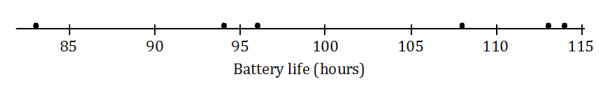
→ The mean was 101 hours. Mark the location of the mean on the dot plot above.
→ What is a typical distance or deviation from the mean for these Brand A batteries?
→ A typical deviation is around 10 hours.
→ Now let’s explore a more common measure of deviation from the mean—the standard deviation.

Walk students through the steps in their lesson resources for Example 1.

How do you measure variability of this data set? One way is by calculating standard deviation.
→ First, find each deviation from the mean.
→ Then, square the deviations from the mean. For example, when the deviation from the mean is -18, the squared deviation from the mean is (-18)²=324.

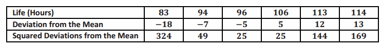
→ Add up the squared deviations:
324+49+25+25+144+169=736.
This result is the sum of the squared deviations.

The number of values in the data set is denoted by n. In this example, n is 6.
→ You divide the sum of the squared deviations by n-1, which here is 6-1, or 5.
\(\frac{736}{5}\)=147.2
→ Finally, you take the square root of 147.2, which to the nearest hundredth is 12.13.

That is the standard deviation! It seems like a very complicated process at first, but you will soon get used to it.

We conclude that a typical deviation of a Brand A battery lifetime from the mean battery lifetime for Brand A is 12.13 hours. The unit of standard deviation is always the same as the unit of the original data set. So, the standard deviation to the nearest hundredth, with the unit, is 12.13 hours. How close is the answer to the typical deviation that you estimated at the beginning of the lesson?

→ How close is the answer to the typical deviation that you estimated at the beginning of the lesson?
→ It is fairly close to the typical deviation of around 10 hours.

The value of 12.13 could be considered to be reasonably close to the earlier estimate of 10. The fact that the standard deviation is a little larger than the earlier estimate could be attributed to the effect of the point at 83. The standard deviation is affected more by values with comparatively large deviations from the mean than, for example, is the mean absolute deviation that students learned about in Grade 6.

This is a good time to mention precision when calculating the standard deviation. Encourage students, when calculating the standard deviation, to use several decimal places in the value that they use for the mean. Explain that students might get somewhat varying answers for the standard deviation depending on how far they round the value of the mean.

Eureka Math Algebra 1 Module 2 Lesson 5 Exercise Answer Key

Exercises 1–5
Now you can calculate the standard deviation of the lifetimes for the eight Brand B batteries. The mean was 100.5.
We already have the deviations from the mean.

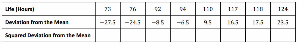
Answer:

Exercise 1.
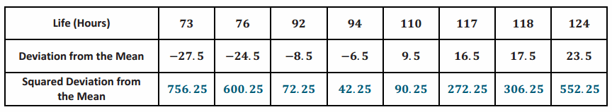
Write the squared deviations in the table.
Answer:
See table above.

Exercise 2.
Add up the squared deviations. What result do you get?
Answer:
The sum is 2,692.

Exercise 3.
What is the value of n for this data set? Divide the sum of the squared deviations by n-1, and write your answer below. Round your answer to the nearest thousandth.
Answer:
n=8; \(\frac{2692}{7}\)≈384.571

Exercise 4.
Take the square root to find the standard deviation. Record your answer to the nearest hundredth.
Answer:
\(\sqrt{384.571}\)≈19.61

Exercise 5.
How would you interpret the standard deviation that you found in Exercise 4? (Remember to give your answer in the context of this question. Interpret your answer to the nearest hundredth.)
Answer:
The standard deviation, 19.61 hours, is a typical deviation of a Brand B battery lifetime from the mean battery lifetime for Brand B.

→ So, now we have computed the standard deviation of the data on Brand A and of the data on Brand B. Compare the two, and describe what you notice in the context of the problem.
→ The fact that the standard deviation for Brand B is greater than the standard deviation for Brand A tells us that the battery life of Brand B had a greater spread (or variability) than the battery life of Brand A. This means that the Brand B battery lifetimes tended to vary more from one battery to another than the battery lifetimes for Brand A.

Exercises 6–7
Jenna has bought a new hybrid car. Each week for a period of seven weeks, she has noted the fuel efficiency (in miles per gallon) of her car. The results are shown below.

Exercise 6.
Calculate the standard deviation of these results to the nearest hundredth. Be sure to show your work.
Answer:
The mean is 44.
The deviations from the mean are 1, 0, -1, 0, 1, 0, -1.
The squared deviations from the mean are 1, 0, 1, 0, 1, 0, 1.
The sum of the squared deviations is 4.
n=7; \(\frac{4}{6}\)≈0.667
The standard deviation is √(0.667) which is approximately 0.82 miles per gallon.

Exercise 7.
What is the meaning of the standard deviation you found in Exercise 6?
Answer:
The standard deviation, 0.82 miles per gallon, is a typical deviation of a weekly fuel efficiency value from the mean weekly fuel efficiency.

→ Why do we take the square root?
→ Before taking the square root, we have a typical squared deviation from the mean. It is easier to interpret a typical deviation from the mean than a typical squared deviation from the mean because a typical deviation has the same units as the original data. For example, the typical deviation from the mean for the battery life data is expressed in hours rather than hours2.
→ Why did we divide by n-1 instead of n?
→ We only use n-1 when we are calculating the standard deviation using sample data. Careful study has shown that using n-1 gives the best estimate of the standard deviation for the entire population. If we have data from an entire population, we would divide by n instead of n-1. (See note below for a detailed explanation.)
NOTE: This topic is addressed throughout a study of statistics:

More information on why to divide by n-1 and not n:

It is helpful to first explore the variance. The variance of a set of values is the square of the standard deviation. So, to calculate the variance, the same process is used, but the square root is not taken at the end.
Suppose, for a start, that there is a very large population of values, for example, the heights of all the people in a country. One can think of the variance of this population as being calculated using a division by n (although, since the population is very large, the difference between using n or n-1 for the population is extremely small).

Imagine now taking a random sample from the population, such as taking a random sample of people from the country and measuring their heights. Use the variance of the sample as an estimate of the variance of the population. If division by n is used in calculating the variance of the sample, the result tends to be a little too small as an estimate of the population variance. (To be a little more precise about this, the sample variance would sometimes be smaller and sometimes larger than the population variance. But, on average, over all possible samples, the sample variance is a little too small.)

So, something has to be done about the formula for the sample variance in order to fix this problem of its tendency to be too small as an estimate of the population variance. It turns out, mathematically, that replacing the n with n-1 has exactly the desired effect. Now, when dividing by n-1, rather than n, even though the sample variance is sometimes greater and sometimes less than the population variance, on average, the sample variance is correct as an estimator of the population variance.

→ What does standard deviation measure? How can we summarize what we are attempting to compute?
→ The value of the standard deviation is close to the average distance of observations from the mean. It can be interpreted as a typical deviation from the mean.
→ How does the spread of the distribution relate to the value of the standard deviation?
→ The larger the spread of the distribution, the larger the standard deviation.
→ Who can write a formula for standard deviation, s?
→ Encourage students to attempt to write the formula without assistance, perhaps comparing their results with their peers.
s=\(\sqrt{\frac{\sum(x-\bar{x})^{2}}{n-1}}\)

In this formula,
→ x is a value from the original data set;
→ x-\(\bar{x}\) is a deviation of the value, x, from the mean, \(\bar{x}\);
→ (x-\(\bar{x}\))² is a squared deviation from the mean;
→ ∑(x-\(\bar{x}\))² is the sum of the squared deviations;
→ \(\frac{\sum(x-\bar{x})^{2}}{n-1}\) is the result of dividing the sum of the squared deviations by n-1;
→ So, \(\sqrt{\frac{\sum(x-\bar{x})^{2}}{n-1}}\) is the standard deviation.

Eureka Math Algebra 1 Module 2 Lesson 5 Problem Set Answer Key

Question 1.
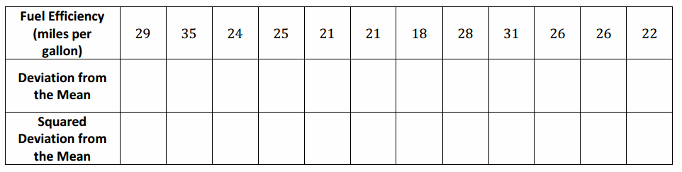
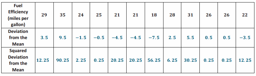
A small car dealership tests the fuel efficiency of sedans on its lot. It chooses 12 sedans for the test. The fuel efficiency (mpg) values of the cars are given in the table below. Complete the table as directed below.

Answer:

a. Calculate the mean fuel efficiency for these cars.
Answer:
Mean =25.5

b. Calculate the deviations from the mean, and write your answers in the second row of the table.
Answer:
See table above.

c. Square the deviations from the mean, and write the squared deviations in the third row of the table.
Answer:
See table above.

d. Find the sum of the squared deviations.
Answer:
The sum of the squared deviations is 251.

e. What is the value of n for this data set? Divide the sum of the squared deviations by n-1.
Answer:
n=12
\(\frac{251}{11}\)=22.818, to the nearest thousandth.

f. Take the square root of your answer to part (e) to find the standard deviation of the fuel efficiencies of these cars. Round your answer to the nearest hundredth.
Answer:
\(\sqrt{22.818}\)=4.78
The standard deviation of the fuel efficiencies of these cars is 4.78 miles per gallon.

Question 2.
The same dealership decides to test fuel efficiency of SUVs. It selects six SUVs on its lot for the test. The fuel efficiencies (in miles per gallon) of these cars are shown below.

Calculate the mean and the standard deviation of these values. Be sure to show your work, and include a unit in your answer.
Answer:
Mean =24.17 miles per gallon; standard deviation =3.97 miles per gallon
Note: Students might get somewhat varying answers for the standard deviation depending on how far they round the value of the mean. Encourage students, when calculating the standard deviation, to use several decimal places in the value that they use for the mean.

Question 3.
Consider the following questions regarding the cars described in Problems 1 and 2.
a. What is the standard deviation of the fuel efficiencies of the cars in Problem 1? Explain what this value tells you.
Answer:
The standard deviation for the cars in Problem 1 is 4.78 miles per gallon. This is a typical deviation from the mean for the fuel efficiencies of the cars in Problem 1.

b. You also calculated the standard deviation of the fuel efficiencies for the cars in Problem 2. Which of the two data sets (Problem 1 or Problem 2) has the larger standard deviation? What does this tell you about the two types of cars (sedans and SUVs)?
Answer:
The standard deviation is greater for the cars in Problem 1. This tells us that there is greater variability in the fuel efficiencies of the cars in Problem 1 (the sedans) than in the fuel efficiencies of the cars in Problem 2 (the SUVs). This means that the fuel efficiency varies more from car to car for sedans than for SUVs.

Eureka Math Algebra 1 Module 2 Lesson 5 Exit Ticket Answer Key

Question 1.
Look at the dot plot below.

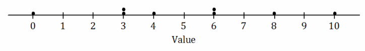
a. Estimate the mean of this data set.
Answer:
The mean of the data set is 5, so any number above 4 and below 6 would be acceptable as an estimate of the mean.

b. Remember that the standard deviation measures a typical deviation from the mean. The standard deviation of this data set is either 3.2, 6.2, or 9.2. Which of these values is correct for the standard deviation?
Answer:
The greatest deviation from the mean is 5 (found by calculating 10-5 or 0-5), and a typical deviation from the mean must be less than 5. So, 3.2 must be chosen as the standard deviation.

Question 2.
Three data sets are shown in the dot plots below.

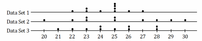
a. Which data set has the smallest standard deviation of the three? Justify your answer.
Answer:
Data Set 1
The points are clustered more closely together in Data Set 1. The deviations or the distances of the points to the left and to the right of the mean position would be smaller for this data set. As a result, the sum of the squares of the distances would also be smaller; thus, the standard deviation would be smaller.

b. Which data set has the largest standard deviation of the three? Justify your answer.
Answer:
Data Set 2
The points of this data set are the most spread out. The deviations or the distances of the points to the left and to the right of the mean position would be larger for this data set. The sum of the squares of the distances would also be larger. As a result, the standard deviation would be larger.