Engage NY Eureka Math Algebra 2 Module 4 Lesson 14 Answer Key
Eureka Math Algebra 2 Module 4 Lesson 14 Example Answer Key
Example 1: Polls
A recent poll stated that 40% of Americans pay ‘a great deal” or a ‘fair amount” of attention to the nutritional information that restaurants provide. This poll was based on a random sample of 2,027 adults living in the United States.
The 40% corresponds to a proportion of 0.40, and 0.40 is called a sample proportion. It is an estimate of the proportion of all adults who would say they pay “a great deal” or a “fair amount” of attention to the nutritional information that restaurants provide.
If you were to take a random sample of 20 Americans, how many would you predict would say that they pay attention to nutritional information? In this lesson, you will investigate this question by generating distributions of sample proportions and investigating patterns in these distributions.
Your teacher will give your group a container of dried beans. Some of the beans in the container are black. With your classmates, you are going see what happens when you take a sample of beans from the container and use the proportion of black beans in the sample to estimate the proportion of black beans in the container (a population proportion).
Exploratory Challenge 1/Exercises 1-9:
Exercise 1.
Each person in the group should randomly select a sample of 20 beans from the container by carefully mixing all the beans and then selecting one bean and recording its color. Replace the bean, mix the bag, and continue to select one bean at a time until 20 beans have been selected. Be sure to replace each bean and mix the bag before selecting the next bean. Count the number of black beans in your sample of 20.
Answer:
Answers will vary, but the number of black beans will center around 8.
Exercise 2.
What is the proportion of black beans in your sample of 20? (Round your answer to 2 decimal places.) This value is called the sample proportion of black beans.
Answer:
Answers will vary, but the sample proportions will center around 0.4.
Exercise 3.
Write your sample propomon on a sticky note, and place the note on the number line that your teacher has drawn on the board. Place your note above the value on the number line that corresponds to your sample proportion.
Answer:
Class data will vary. One possible sampling distribution is shown below.
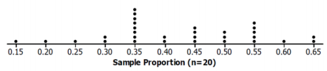
The graph of all the students’ sample proportions is called the sampling distribution of the samples’ proportions. This sampling distribution is an approximation of the actual sampling distribution of all possible samples of size 20.
Exercise 4.
Describe the shape of the distribution.
Answer:
Answers might vary, but the shape is generally mound-shaped.
Exercise 5.
What was the smallest sample proportion observed?
Answer:
Answers will vary. Based on the sample graph: 0.15
Exercise 6.
What was the largest sample proportion observed?
Answer:
Answers will vary. Based on the sample graph: 0.65
Exercise 7.
What sample proportion occurred most often?
Answer:
Answers will vary, but the sample proportion should be around 0.4. Based on the sample graph: 0.35
Exercise 8.
Using technology, find the mean and standard deviation of the sample proportions used to construct the sampling distribution created by the class.
Answer:
Answers will vary, but the mean will be approximately 0.4, and the standard deviation will be approximately 0.11.
Exercise 9.
How does the mean of the sampling distribution compare with the population proportion of 0.40?
Answer:
Answers will vary, but the two values should be about the same. In theory, the mean of the sampling distribution of sample proportions is equal to the population proportion.
Example 2: Sampling Variability
What do you think would happen to the sampling distribution if everyone in the class took a random sample of 40 beans from the container? To help answer this question, you will repeat the process described in Example 1, but this time you will draw a random sample of 40 beans instead of 20.
Exploratory Challenge 2/Exercises 10 – 21:
Exercise 10.
Take a random sample with the replacement of 40 beans from the container. Count the number of black beans in your sample of 40 beans.
Answer:
Answers will vary, but the number of black beans will center around 16.
Exercise 11.
What is the proportion of black beans in your sample of 40? (Round your answer to 2 decimal places.)
Answer:
Answers will vary, but the sample proportions will center around 0.40.
Exercise 12.
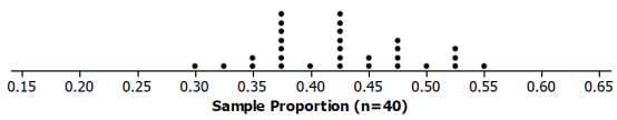
Write your sample proportion on a sticky note, and place It on the number line that your teacher has drawn on the board. Place your note above the value on the number line that corresponds to your sample proportion.
Answer:
Class data will vary. One possible sampling distribution is shown below.
Exercise 13.
Describe the shape of the distribution.
Answer:
Answers may vary, but the shape is generally mound-shaped.
Exercise 14.
What was the smallest sample proportion observed?
Answer:
Answers will vary. Based on the sample graph: 0.30
Exercise 15.
What was the largest sample proportion observed?
Answer:
Answers will vary. Based on the sample graph: 0. 55
Exercise 16.
What sample proportion occurred most often?
Answer:
Answer will vary but will be approximately 0.4.
Exercise 17.
Using technology, find the mean and standard deviation of the sample proportions used to construct the sampling distribution created by the class.
Answer:
Answers will vary, but the mean will be approximately 0.4 and the standard deviation approximately 0.08.
Exercise 18.
How does the mean of the sampling distribution compare with the population proportion of 0.40?
Answer:
Answers will vary, but the two values should be about the same. In theory, the mean of the sampling distribution of sample proportions is equal to the population proportion.
Exercise 19.
How does the mean of the sampling distribution based on random samples of size 20 compare to the mean of the sampling distribution based on random samples of size 40?
Answer:
The two means are approximately the same, about 0.4.
Exercise 20.
As the sample size increased from 20 to 40, describe what happened to the sampling variability (standard deviation of the distribution of sample proportions)?
Answer:
The standard deviation of the distribution of the sample proportions based on a sample size of 40 is less than the standard deviation of the distribution of the sample proportions based on a sample size of 20.
Exercise 21.
What do you think would happen to the variability (standard deviation) of the distribution of sample proportions if the sample size for each sample was 80 instead of 40? Explain.
Answer:
Because the standard deviation decreased as sample size increased from 20 to 40, I expect that the standard deviation will decrease further when the sample size is 80.
Eureka Math Algebra 2 Module 4 Lesson 14 Problem Set Answer Key
Question 1.
A class of 28 eleventh graders wanted to estimate the proportion of all juniors and seniors at their high school with part-time jobs after school. Each eleventh grader took a random sample of 30 juniors and seniors and then calculated the proportion with part-time jobs. Following are the 28 sample proportions.
0.7, 0.8, 0.57, 0.63, 0.7, 0.47, 0.67, 0.67, 0.8, 0.77, 0.4, 0.73, 0.63, 0.67, 0.6, 0.77, 0.77, 0.77, 0.53, 0.57, 0.73, 0.7, 0.67, 0.7, 0.77, 0.57, 0.77, 0.67
a. Construct a dot plot of the sample proportions.
Answer:
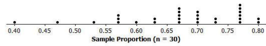
b. Describe the shape of the distribution.
Answer:
Skewed to the left
c. Using technology, find the mean and standard deviation of the sample proportions.
Answer:
Mean= 0.67
Standard deviation = 0. 1
d. Do you think that the proportion of all juniors and seniors at the school with part-time jobs could be 0.7? Do you think it could be 0.5? Justify your answers based on your dot plot.
Answer:
It is likely that the proportion of all juniors and seniors with part-time jobs could be 0.70 since 0.70 is near the center of the dot plot. It is unlikely that the proportion of all juniors and seniors Is 0.5 since there are very few samples with a sample proportion of 0.5 or less.
e. Suppose the eleventh graders had taken random samples of size 60. How would the distribution of sample proportions based on samples of size 60 differ from the distribution for samples of size 30?
Answer:
The sampling distribution would be mound-shaped with approximately the same mean of the sampling distribution based on size 30, but the standard deviation of the sampling distribution based on size 60 would be smaller than one based on samples of size 30.
Question 2.
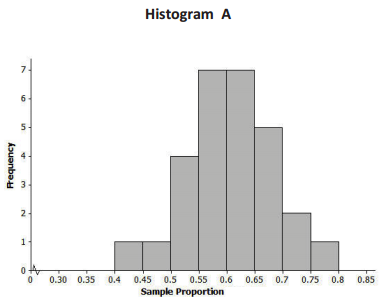
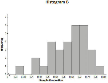
A group of eleventh graders wanted to estimate the proportion of all students at their high school who suffer from allergies. Each student in one group of eleventh graders took a random sample of 20 students, while each student in another group of eleventh graders each took a random sample of 40 students. Below are the two sampling distributions (shown as histograms) of the sample proportions of high school students who said that they suffer from allergies. Which histogram is based on random samples of size 40? Explain.
Answer:
Histogram A is based on random samples of size 40 because it has less variability than Histogram B.
Question 3.
The nurse in your school district would like to study the proportion of all high school students in the district who usually get at least eight hours of sleep on school nights. Suppose each student in your class takes a random sample of 20 high school students in the district and each calculates their sample proportion of students who said that they usually get at least eight hours of sleep on school nights. Below is a histogram of the sampling distribution.
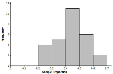
a. Do you think that the proportion of all high school students who usually get at least eight hours of sleep on school nights could have been 0.4? Do you think It could have been 0.55? Could It have been 0.75? Justify your answers based on the histogram.
Answer:
The proportion of all high school students who usually get at least eight hours of sleep is likely around 0.4 since that is near the center of the sampling distribution. The proportion could be 0.55 since that is still close to the center of the distribution. It is unlikely that the proportion of all high school students is 0.75 since none of the samples produced sample proportions as large as 0.75.
b. Suppose students had taken random samples of size 60. How would the distribution of sample proportions based on samples of size 60 differ from those of size 20?
Answer:
The means of the two distributions would be relatively close, but the standard deviation of the distribution based on samples of size 60 would be smaller than the standard deviation of the distribution based on sample sizes of 20.
Eureka Math Algebra 2 Module 4 Lesson 14 Exit Ticket Answer Key
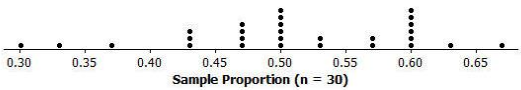
A group of eleventh graders wanted to estimate the population proportion of students in their high school who drink at least one soda per day. Each student selected a different random sample of 30 students from the high school and calculated the proportion that drinks at least one soda per day. The dot plot below shows the sampling distribution. This distribution has a mean of 0.51 and a standard deviation of 0.09.
Question 1.
Describe the shape of the distribution.
Answer:
Approximately symmetric centered around 0.50
Question 2.
What is your estimate for the proportion of all students who would report that they drink at least one soda per day?
Answer:
0.51, which is the mean of the sampling distribution
Question 3.
If, instead of taking random samples of 30 students in the high school, the eleventh graders randomly selected samples of size 60, describe what will happen to the standard deviation of the sampling distribution of the sample proportions.
Answer:
The standard deviation will decrease.