Engage NY Eureka Math Algebra 2 Module 1 Lesson 15 Answer Key
Eureka Math Algebra 2 Module 1 Lesson 15 Example Answer Key
Example 1
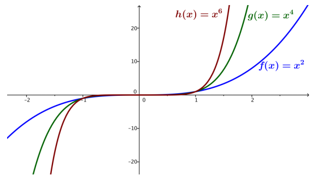
Sketch the graph of f(x) = x3. What will the graph of g(x) = x5 look like? Sketch this on the same coordinate plane. What will the graph of h(x) = x7 look like? Sketch this on the same coordinate plane.
Answer:
Have students recall and sketch the graph of f(x) = x3. Discuss the characteristics of the graph, where the x-intercept is, and why the graph is above the x-axis for x > 0 and below the x-axis for x < 0.
In pairs or in groups, have students discuss or write what they think the graph of g(x) = x5 will look like and how it will relate to the graph of f(x) = x3. They should sketch their results on top of the original graph of f. Discuss with students what they have sketched, and emphasize the similarities to the graph of f(x) = x3.
Finally, in pairs or in groups, have students discuss or write what they think the graph of h(x) = x7 will look like and how it will relate to the graphs of f and g. They should sketch on the same graph they used with the previous two graphs. Again, discuss the graphs with students, and emphasize the similarities between graphs.
Using a graphing utility, have students graph all three functions simultaneously to confirm their sketches.
Ask students to compare and describe the behavior of the value of f(x) as the absolute value of x increases without bound. Guide them to use the terminology of the end behavior of the function.
Ask students to make a generalization about the end behavior of polynomials of odd degree individually or with a partner. After students have generalized the end behavior, have them create their own graphic organizer like the following.

If students suspect that polynomial functions with odd degree always have the value of the function increase as x increases, then suggest examining a function with a negative leading coefficient, such as f(x) = 4 – x or g(x) = – x3.
Eureka Math Algebra 2 Module 1 Lesson 15 Opening Exercise Answer Key
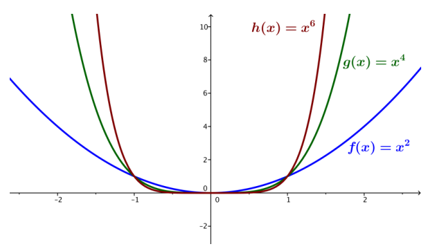
Sketch the graph of f(x) = x2. What will the graph of g(x) = x4 look like? Sketch it on the same coordinate plane. What will the graph of h(x) = x6 look like?
Answer:
Have students recall and sketch the graph of f(x) = x2. Discuss the characteristics of the graph, where the x-intercept is, and why the graph stays above the x-axis on either side of the x-intercept.
In pairs or in groups, have them discuss or write what they think the graph of g(x) = x4 will look like and how they think it compares to the graph of f(x) = x2. 0nce they do so, they should sketch their idea of the graph of g on top of the graph of f. Discuss with students what they have sketched, and emphasize the similarities between the two graphs.
Since g(x) = (x2)2, g(x) will increase faster as x increases than f(x) does. Both graphs pass through (0, 0). The basic shapes are the same, but near the origin the graph of g is flatter than the graph of f.
Finally, in pairs or in groups, have students discuss or write what they think the graph of h(x) = x6 will look like and how they think it will compare to graphs of f and g. 0nce they do so, students should sketch on the same graph the previous two graphs. Again, discuss graphs with students, and emphasize the similarities between graphs.
Since h(x) = x2 ∙ x2 ∙ x2, the graph of h again passes through the origin. Since we are squaring and multiplying by squares, the graph of h should look about the same as the graphs off and g but increase even faster and be even flatter near the origin.
→ Using a graphing utility, have students graph all three functions simultaneously to confirm their sketches.
Eureka Math Algebra 2 Module 1 Lesson 15 Exercise Answer Key
Exercise 1.
a. Consider the following function, f(x) = 2x4+ x3 – x2 + 5x + 3, with a mixture of odd and even degree terms. Predict whether its end behavior will be like the functions in the Opening Exercise or more like the functions from Example 1. Graph the function f using a graphing utility to check your prediction.
Answer:
Students see that this function acts more like the even-degree monomial functions from the Opening Exercise.
b. Consider the following function, f(x) = 2x5 – x4 – 2x3 + 4x2 + x + 3, with a mixture of odd and even
degree terms. Predict whether its end behavior will be like the functions in the Opening Exercise or more like the functions from Example 1. Graph the function f using a graphing utility to check your prediction.
Answer:
Students see that this function acts more like odd-degree monomial functions from Example 1. They can draw a conclusion such as that the function behaves like the highest degree term.
c. Thinking back to our discussion of x-intercepts of graphs of polynomial functions from the previous lesson, sketch a graph of an even-degree polynomial function that has no x-Intercepts.
Answer:
Students may draw the graph of a quadratic function that stays above the x-axis such os the graph of
f(x) = x2 + 1.
d. Similarly, can you sketch a graph of an odd-degree polynomial function with no x-intercepts?
Answer:
Have students work in pairs or groups and discover that because of the “cut through” nature of graphs of odd-degree polynomial function there is always an x-intercept.
Conclusion: Graphs of odd-powered polynomial functions always have an x-intercept, which means that odd-degree polynomial functions always have at least one zero (or root) and that polynomial functions of odd-degree always have opposite end behaviors as x → ∞ and x → ∞.
Exercise 2.
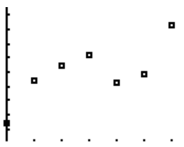
The Center for Transportation Analysis (CTA) studies all aspects of transportation in the United States, from energy and environmental concerns to safety and security challenges. A 1997 study compiled the following data of the fuel economy in miles per gallon (mpg) of a car or light truck at various speeds measured in miles per hour (mph). The data are compiled in the table below.
Fuel Economy by speed
| Speed (mph) | Fuel Economy (mpg) |
| 15 | 24.4 |
| 20 | 27.9 |
| 25 | 30.5 |
| 30 | 31.7 |
| 35 | 31.2 |
| 40 | 31.0 |
| 45 | 31.6 |
| 50 | 32.4 |
| 55 | 32.4 |
| 60 | 31.4 |
| 65 | 29.2 |
| 70 | 26.8 |
| 75 | 24.8 |
![]()
a. Plot the data using a graphing utility. Which variable is the independent variable?
Answer:
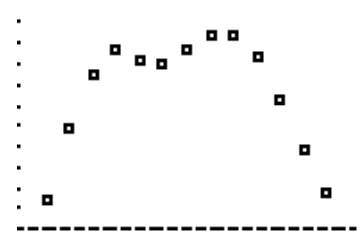
Speed is the independent variable.
b. This data can be modeled by a polynomial function. Determine if the function that models the data would have an even or odd degree.
Answer:
It seems we could model this data by on even-degree polynomial function.
c. Is the leading coefficient of the polynomial that can be used to model this data positive or negative?
Answer:
The leading coefficient would be negative since the end behavior of this function is to approach negative infinity on both sides.
d. List two possible reasons the data might have the shape that it does.
Answer:
Possible responses: Fuel economy improves up to a certain speed, but then wind resistance at higher speeds reduces fuel economy; the increased gas needed to go higher speeds reduces fuel economy.
Eureka Math Algebra 2 Module 1 Lesson 15 Problem Set Answer Key
Question 1.
Graph the functions from the Opening Exercise simultaneously using a graphing utility and zoom in at the origin.
a. At x = 0. 5, order the values of the functions from least to greatest.
Answer:
At x = 0.5, x6 < x4 < x2.
b. At x = 2. 5, order the values of the functions from least to greatest.
Answer:
At x = 2.5, x2 < x 4 < x6.
c. Identify the x-value(s) where the order reverses. Write a brief sentence on why you think this switch occurs.
Answer:
At x = 1 and x = – 1, the values of the functions are equal Students may write that when a number between 0 and 1 is taken to higher even powers, it gets smaller, and when a number greater than 1 is taken to higher even powers, it gets larger, and when a negative number is raised to an even power it becomes positive. So for – 1 < x < 0 the behavior is the same as for 0 < x < 1.
Question 2.
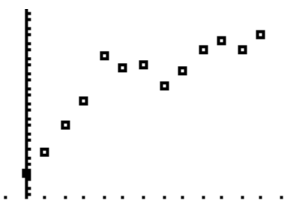
The National Agricultural Statistics Service (NASS) is an agency within the USDA that collects and analyzes data covering virtually every aspect of agriculture in the United States. The following table contains information on the amount (in tons) of the following vegetables produced in the U.S. from 1988 – 1994 for processing into canned, frozen, and packaged foods: lima beans, snap beans, beets, cabbage, sweet corn, cucumbers, green peas, spinach, and tomatoes.
Vegetable Production by Year
| Year | Vegetable Production (tons) |
| 1988 | 11,393,320 |
| 1989 | 14,450,970 |
| 1990 | 15,444,970 |
| 1991 | 16,151,030 |
| 1992 | 14,236,320 |
| 1993 | 14,904,750 |
| 1994 | 18,313,150 |
![]()
a. Plot the data using a graphing utility.
Answer:
b. Determine if the data display the characteristics of an odd- or even-degree polynomial function.
Answer:
Looking at the end behavior, the data show the characteristics of an odd-degree polynomial function.
c. List two possible reasons the data might have such a shape.
Answer:
Possible responses: Bad weather in 1992 and 1993; shifts in demand for fresh foods vs. processed.
Question 3.
The U.S. Energy Information Administration (EIA) Is responsible for collecting and analyzing information about energy production and use in the United States and for informing policy makers and the public about issues of energy, the economy, and the environment. The following table contains data from the EIA about natural gas consumption from 1950 – 2010, measured in millions of cubic feet.
U.S. Natural Gas Consumption by year
| Year |
U.S. natural gas total consumption |
| 1950 | 5.77 |
| 1955 | 8.69 |
| 1960 | 11.97 |
| 1965 | 15.28 |
| 1970 | 21.14 |
| 1975 | 19.54 |
| 1980 | 19.88 |
| 1985 | 17.28 |
| 1990 | 19.17 |
| 1995 | 22.21 |
| 2000 | 23.33 |
| 2005 | 22.01 |
| 2010 | 24.09 |
![]()
a. Plot the data using a graphing utility.
Answer:
b. Determine If the data display the characteristics of an odd- or even-degree polynomial function.
Answer:
Looking at the end behavior, the data show the characteristics of an odd-degree polynomial function.
c. List two possible reasons the data might have such a shape.
Answer:
Possible responses: changes in supply, new sources and technology created new supplies, weather may impact usage.
Question 4.
We use the term even function when a function f satisfies the equation f(- x) = f(x) for every number x in its domain. Consider the function f(x) = – 3x2 + 7. Note that the degree of the function is even, and each term is of an even degree (the constant term is degree 0).
a. Graph the function using a graphing utility.
Answer:
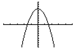
b. Does this graph display any symmetry?
Answer:
Yes, it is symmetric about the y-axis.
c. Evaluate f(- x).
Answer:
f(-x) = – 3(- x)2 + 7 = – 3x2 + 7
d. Is f an even function? Explain how you know.
Answer:
Yes, because f(- x) = – 3x2 + 7 = f(x) for all real values of x.
Question 5.
We use the term odd function when a function f satisfies the equation f(- x) = – f(x) for every number x in its domain. Consider the function f(x) = 3x3 – 4x. The degree of the function is odd, and each term is of an odd degree.
a. Graph the function using a graphing utility.
Answer:
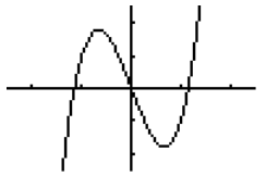
b. Does this graph display any symmetry?
Answer:
Yes, but not the same as in part (a). This graph is symmetric about the origin. We can see this because if the graph is rotated 180° about the origin, it appears to be unchanged.
c. Evaluate f(-x).
Answer:
f(- x) = 3(- x)3 – 4(- x) = – 3x3 + 4x
d. Is f an odd function? Explain how you know.
Answer:
Yes, we know because f(- x) = – 3x3 + 4x = – (3x3 – 4x) = – f (x) for all real values of x.
Question 6.
We have talked about x-intercepts of the graph of a function in both this lesson and the previous one. The x-intercepts correspond to the zeros of the function. Consider the following examples of polynomial functions and their graphs to determine an easy way to find the y-intercept of the graph of a polynomial function.
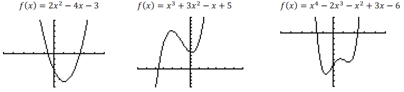
Answer:
The y-intercept is the value where the graph of a function f intersects the y-axis, if 0 is in the domain off. Therefore, for a function f whose domain and range are a subset of the real numbers, the y-intercept is f(0). For polynomial functions, f(0) is easy to determine – it is just the constant term when the polynomial function is written in standard form.
Eureka Math Algebra 2 Module 1 Lesson 15 Exit Ticket Answer Key
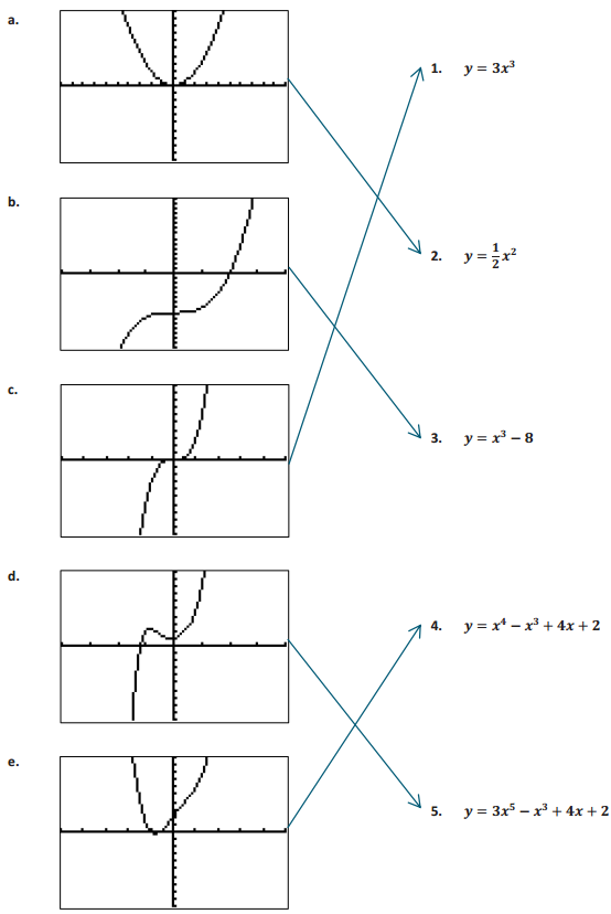
Without using a graphing utility, match each graph below ¡n column 1 with the function in column 2 that it represents.
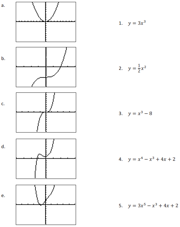
Answer: