Students can use the Spectrum Math Grade 8 Answer Key Chapter 6 Lesson 6.4 Creating Equations to Solve Bivariate Problems as a quick guide to resolve any of their doubts
Spectrum Math Grade 8 Chapter 6 Lesson 6.4 Creating Equations to Solve Bivariate Problems Answers Key
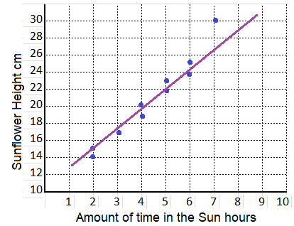
When given a set of bivariate data with a fairly consistent rate of change, a scatter plot with a trend line can be used to create an equation that will approximate the relationship between the two sets of data.
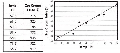
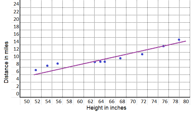
m = \(\frac{522-406}{71.8-65.3}\) = \(\frac{116}{6.5}\) = 17.85
y = 17.85x – 759.61
406 = (17.85)(65.3) + b
b = -759.61
Step 1: Use the data set to create a scatter plot with a trend line.
Step 2: Use the 2 points of data closest to the trend line to find the slope of the trend line.
Step 3: Use one point of data with the calculated slope to find the y-intersect of the trend line.
Step 4: Use the calculated slope and y-intersect to state the equation in linear form, y = mx + b.
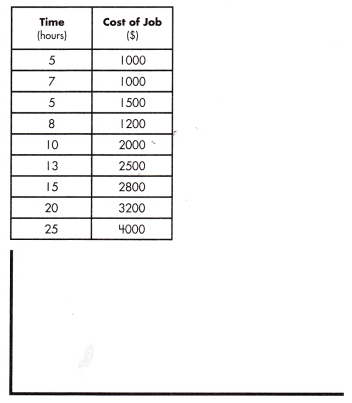
Use each set of bivariate data to create a scatter plot, trend line, and an equation that approximates the data set.
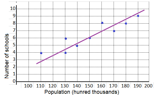
Question 1.
a.
equation: ______________
Answer:
equation: y = 5.5 x – 4.5
Explanation:
We know that,
When given a set of bivariate data with a fairly consistent rate of change,
a scatter plot with a trend line can be used to create an equation that will approximate the relationship between the two sets of data.
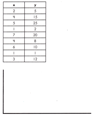
m = \(\frac{12 – 1}{3 – 1}\) = \(\frac{11}{2}\) = 5.5
y = 5.5 x + b
12 = 5.5 (3) + b
b = 12 – 16.5 = – 4.5
y = mx + b
y = 5.5 x – 4.5
b.
equation: ______________
Answer:
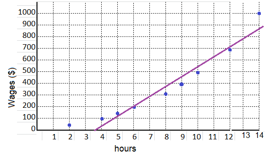
equation: y = 5.5 x – 4.5
Explanation:
We know that,
When given a set of bivariate data with a fairly consistent rate of change,
a scatter plot with a trend line can be used to create an equation that will approximate the relationship between the two sets of data.
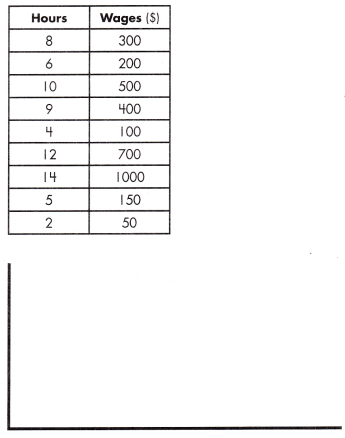
m = \(\frac{1000 – 700}{14 – 12}\) = \(\frac{300}{2}\) = 150
y = 150 x + b
500 = 150 (10) + b
b = 500 – 1500 = – 1000
y = mx + b
y = 150 x – 1000
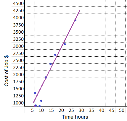
Use each set of bivariate data to create a scatter plot, trend line, and an equation that approximates the data set.
Question 1.
a.
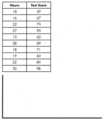
equation: ______________
Answer:
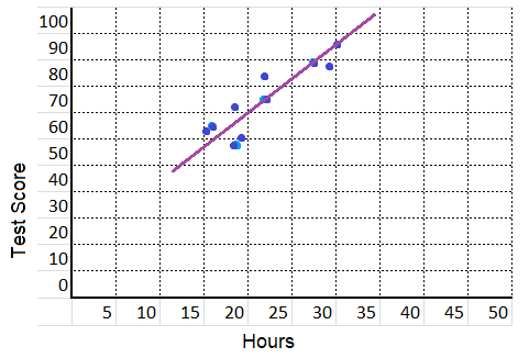
equation: y = 1.75 x – 56.75
Explanation:
We know that,
When given a set of bivariate data with a fairly consistent rate of change,
a scatter plot with a trend line can be used to create an equation that will approximate the relationship between the two sets of data.
m = \(\frac{98 – 84}{30 – 22}\)
= \(\frac{14}{8}\)
= \(\frac{7}{4}\)
= 1.75
y = \(\frac{7}{4}\) x + b
y = 1.75 x + b
90 = \(\frac{7}{4}\) (19) + b
90 = 1.75 (19) + b
b = 90 – 33.25 = 56.75
y = mx + b
y = 1.75 x + 56.75
b.
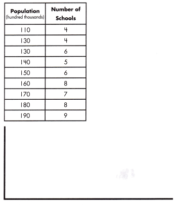
equation: ______________
Answer:
equation:
y = 0.1 x – 10
Explanation:
We know that,
When given a set of bivariate data with a fairly consistent rate of change,
a scatter plot with a trend line can be used to create an equation that will approximate the relationship between the two sets of data.
m = \(\frac{9 – 8}{190 – 180}\)
= \(\frac{1}{10}\)
= 0.1
y = \(\frac{1}{10}\) x + b
y = 0.1 x + b
7 = \(\frac{1}{10}\) (170) + b
7 = 0.1 (170) + b
b = 7 – 17
b = -10
y = mx + b
y = 0.1 x – 10
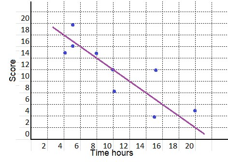
Question 2.
a.
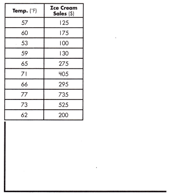
equation: ______________
Answer:
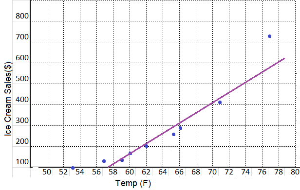
equation:
y = 16.67 x – 783.33
Explanation:
We know that,
When given a set of bivariate data with a fairly consistent rate of change,
a scatter plot with a trend line can be used to create an equation that will approximate the relationship between the two sets of data.
m = \(\frac{175 – 125}{60 – 57}\)
= \(\frac{50}{3}\)
= 16.67
y = \(\frac{50}{3}\) x + b
y = 16.67x + b
100 = \(\frac{130}{6}\) (53) + b
100 = 16.67 (53) + b
b = 100 – 883.33
b = -783.33
y = mx + b
y = 16.67 x – 783.33
b.
equation: ______________
Answer:
equation:
y = 2x + 13
Explanation:
We know that,
When given a set of bivariate data with a fairly consistent rate of change,
a scatter plot with a trend line can be used to create an equation that will approximate the relationship between the two sets of data.
m = \(\frac{19 – 15}{4 – 2}\)
= \(\frac{4}{2}\)
= 2
y = 2 x + b
25 = 2(6) + b
b = 13
y = mx + b
y = 2x + 13
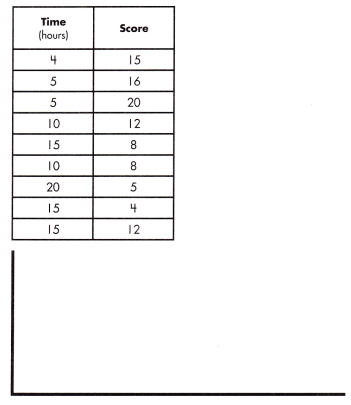
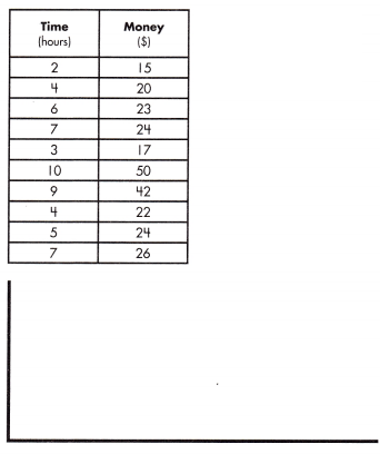
Use each set of bivariate data to create a scatter plot, trend line, and an equation that approximates the data set.
Question 1.
a.
equation: ______________
Answer:
equation:
y = 250x – 500
Explanation:
We know that,
When given a set of bivariate data with a fairly consistent rate of change,
a scatter plot with a trend line can be used to create an equation that will approximate the relationship between the two sets of data.
m = \(\frac{1500 – 1000}{7 – 5}\)
= \(\frac{500}{2}\)
= 250
y = 250 x + b
2000 = 250(10) + b
b = 2000 – 2500
b = -500
y = mx + b
y = 250x – 500
b.
equation: ______________
Answer:
equation:
y = x + 11
Explanation:
We know that,
When given a set of bivariate data with a fairly consistent rate of change,
a scatter plot with a trend line can be used to create an equation that will approximate the relationship between the two sets of data.
m = \(\frac{16 – 15}{5 – 4}\)
= \(\frac{1}{1}\)
= 1
y = mx + b
15 = 1 (4) + b
15 = 4 + b
b = 11
y = mx + b
y = (1)x + 11
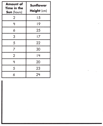
Question 2.
a.
equation: ______________
Answer:
equation:
y = x + 13
Explanation:
We know that,
When given a set of bivariate data with a fairly consistent rate of change,
a scatter plot with a trend line can be used to create an equation that will approximate the relationship between the two sets of data.
m = \(\frac{26 – 24}{7 – 5}\)
= \(\frac{2}{2}\)
= 1
y = m x + b
15 = 1(2) + b
b = 13
y = mx + b
y = x + 13
b.
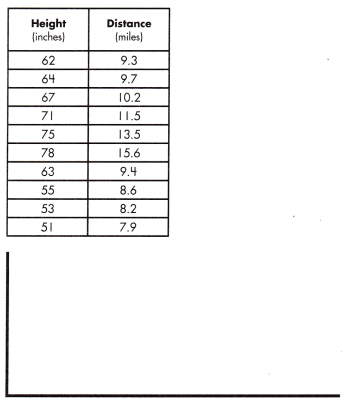
equation: ______________
Answer:
 equation:
y = 50x – 403
Explanation:
We know that,
When given a set of bivariate data with a fairly consistent rate of change,
a scatter plot with a trend line can be used to create an equation that will approximate the relationship between the two sets of data.
m = \(\frac{64 – 62}{9.7 – 9.3}\)
= \(\frac{2}{0.4}\)
= 50
y = m x + b
62 =50(9.3) + b
62 – 465 = b
b = – 403
y = mx + b
y = 50x – 403