Engage NY Eureka Math 8th Grade Module 6 Lesson 9 Answer Key
Eureka Math Grade 8 Module 6 Lesson 9 Exercise Answer Key
Example 1: Crocodiles and Alligators
Scientists are interested in finding out how different species adapt to finding food sources. One group studied crocodilians to find out how their bite force was related to body mass and diet. The table below displays the information they collected on body mass (in pounds) and bite force (in pounds).
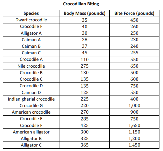
Data Source: http://journals.plos.org/plosone/article?id = 10.1371/journal.pone.0031781#pone – 0031781 – t001
(Note: Body mass and bite force have been converted to pounds from kilograms and newtons, respectively.)
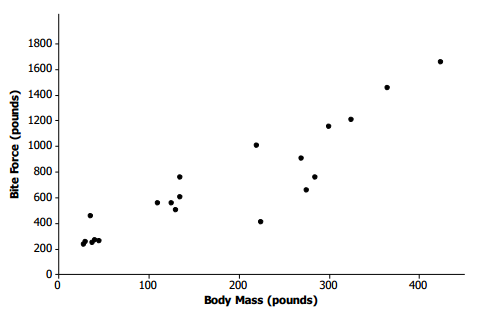
As you learned in the previous lesson, it is a good idea to begin by looking at what a scatter plot tells you about the data. The scatter plot below displays the data on body mass and bite force for the crocodilians in the study.
Exercises 1–6
Exercise 1.
Describe the relationship between body mass and bite force for the crocodilians shown in the scatter plot.
Answer:
As the body mass increases, the bite force tends to also increase.
Exercise 2.
Draw a line to represent the trend in the data. Comment on what you considered in drawing your line.
Answer:
The line should be as close as possible to the points in the scatter plot. Students explored this idea in Lesson 8.
Exercise 3.
Based on your line, predict the bite force for a crocodilian that weighs 220 pounds. How does this prediction compare to the actual bite force of the 220 – pound crocodilian in the data set?
Answer:
Answers will vary. A reasonable prediction is around 650 to 700 pounds. The actual bite force was 1,000 pounds, so the prediction based on the line was not very close for this crocodilian.
Exercise 4.
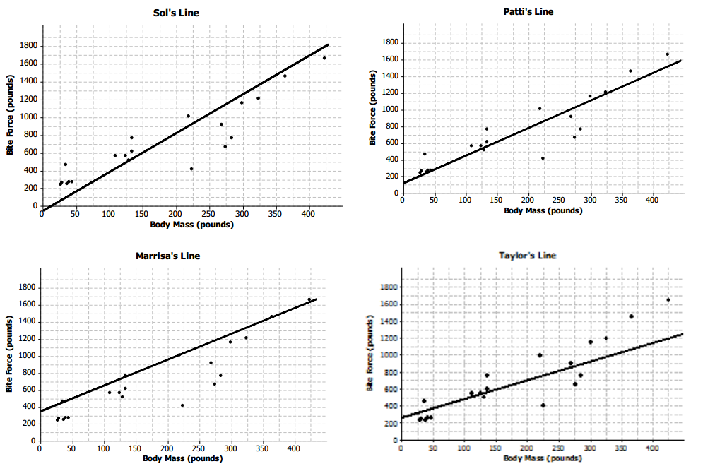
Several students decided to draw lines to represent the trend in the data. Consider the lines drawn by Sol, Patti, Marrisa, and Taylor, which are shown below.
For each student, indicate whether or not you think the line would be a good line to use to make predictions.
Explain your thinking.
a. Sol’s line
Answer:
In general, it looks like Sol’s line overestimates the bite force for heavier crocodilians and underestimates the bite force for crocodilians that do not weigh as much.
b. Patti’s line
Answer:
Patti’s line looks like it fits the data well, so it would probably produce good predictions. The line goes through the middle of the points in the scatter plot, and the points are fairly close to the line.
c. Marrisa’s line
Answer:
It looks like Marrisa’s line overestimates the bite force because almost all of the points are below the line.
d. Taylor’s line
Answer:
It looks like Taylor’s line tends to underestimate the bite force. There are many points above the line.
Exercise 5.
What is the equation of your line? Show the steps you used to determine your line. Based on your equation, what is your prediction for the bite force of a crocodilian weighing 200 pounds?
Answer:
Answers will vary. Students have learned from previous modules how to find the equation of a line. Anticipate students to first determine the slope based on two points on their lines. Students then use a point on the line to obtain an equation in the form y = mx + b (or y = a + bx). Students use their lines to predict a bite force for a crocodilian that weighs 200 pounds. A reasonable answer would be around 800 pounds.
Exercise 6.
Patti drew vertical line segments from two points to the line in her scatter plot. The first point she selected was for a dwarf crocodile. The second point she selected was for an Indian gharial crocodile.
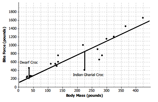
a. Would Patti’s line have resulted in a predicted bite force that was closer to the actual bite force for the dwarf crocodile or for the Indian gharial crocodile? What aspect of the scatter plot supports your answer?
Answer:
The prediction would be closer to the actual bite force for the dwarf crocodile. That point is closer to the line (the vertical line segment connecting it to the line is shorter) than the point for the Indian gharial crocodile.
b. Would it be preferable to describe the trend in a scatter plot using a line that makes the differences in the actual and predicted values large or small? Explain your answer.
Answer:
It would be better for the differences to be as small as possible. Small differences are closer to the line.
Exercise 7: Used Cars
Exercise 7.
Suppose the plot below shows the age (in years) and price (in dollars) of used compact cars that were advertised in a local newspaper.
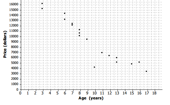
a. Based on the scatter plot above, describe the relationship between the age and price of the used cars.
Answer:
The older the car, the lower the price tends to be.
b. Nora drew a line she thought was close to many of the points and found the equation of the line. She used the points (13,6000) and (7,12000) on her line to find the equation. Explain why those points made finding the equation easy.
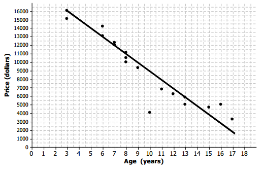
Answer:
The points are at the intersection of the grid lines in the graph, so it is easy to determine the coordinates of these points.
c. Find the equation of Nora’s line for predicting the price of a used car given its age. Summarize the trend described by this equation.
Answer:
Using the points, the equation is y = – 1000x + 19000, or Price = – 1000(age) + 19000. The slope of the line is negative, so the line indicates that the price of used cars decreases as cars get older.
d. Based on the line, for which car in the data set would the predicted value be farthest from the actual value? How can you tell?
Answer:
It would be farthest for the car that is 10 years old. It is the point in the scatter plot that is farthest from the line.
e. What does the equation predict for the cost of a 10 – year – old car? How close was the prediction using the line to the actual cost of the 10 – year – old car in the data set? Given the context of the data set, do you think the difference between the predicted price and the actual price is large or small?
Answer:
The line predicts a 10 – year – old car would cost about $9,000. – 1000(10) + 19000 = 9000. Compared to $4,040 for the 10 – year – old car in the data set, the difference would be $4,960. The prediction is off by about $5,000, which seems like a lot of money, given the prices of the cars in the data set.
f. Is $5,000 typical of the differences between predicted prices and actual prices for the cars in this data set? Justify your answer.
Answer:
No, most of the differences would be much smaller than $5,000. Most of the points are much closer to the line, and most predictions would be within about $1,000 of the actual value.
Eureka Math Grade 8 Module 6 Lesson 9 Problem Set Answer Key
Question 1.
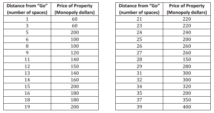
The Monopoly board game is popular in many countries. The scatter plot below shows the distance from “Go” to a property (in number of spaces moving from “Go” in a clockwise direction) and the price of the properties on the Monopoly board. The equation of the line is P = 8x + 40, where P represents the price (in Monopoly dollars) and x represents the distance (in number of spaces).
Price of Property Versus Distance from “Go” in Monopoly
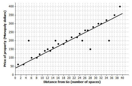
a. Use the equation to find the difference (observed value – predicted value) for the most expensive property and for the property that is 35 spaces from “Go.”
Answer:
The most expensive property is 39 spaces from “Go” and costs $400. The price predicted by the line would be 8(39) + 40, or $352. Observed price – predicted price would be $400 – $352 = $48. The price predicted for 35 spaces from “Go” would be 8(35) + 40, or $320. Observed price – predicted price would be $200 – $320 = – $120.
b. Five of the points seem to lie in a horizontal line. What do these points have in common? What is the equation of the line containing those five points?
Answer:
These points all have the same price. The equation of the horizontal line through those points would be
P = 200.
c. Four of the five points described in part (b) are the railroads. If you were fitting a line to predict price with distance from “Go,” would you use those four points? Why or why not?
Answer:
Answers will vary. Because the four points are not part of the overall trend in the price of the properties, I would not use them to determine a line that describes the relationship. I can show this by finding the total error to measure the fit of the line.
Question 2.
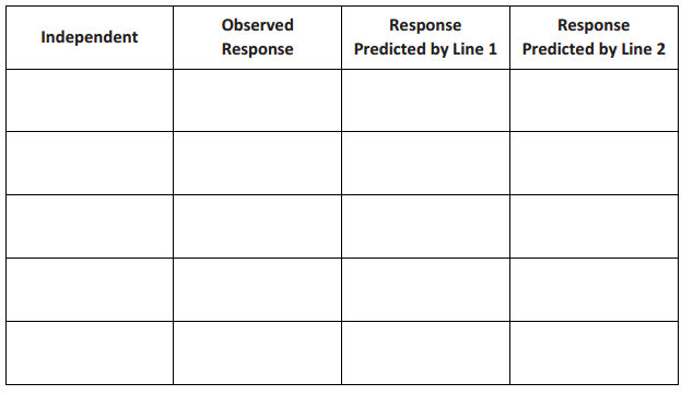
The table below gives the coordinates of the five points shown in the scatter plots that follow. The scatter plots show two different lines.
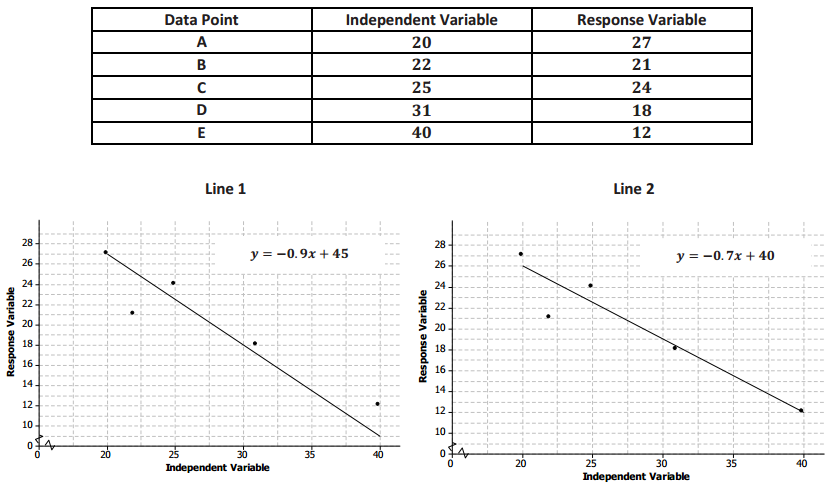
a. Find the predicted response values for each of the two lines.
Answer:
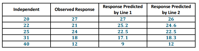
b. For which data points is the prediction based on Line 1 closer to the actual value than the prediction based on Line 2?
Answer:
It is only for data point A. For data point C, both lines are off by the same amount.
c. Which line (Line 1 or Line 2) would you select as a better fit? Explain.
Answer:
Line 2 is a better fit because it is closer to more of the data points.
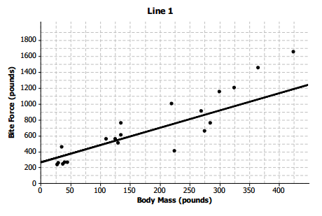
Question 3.
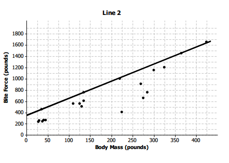
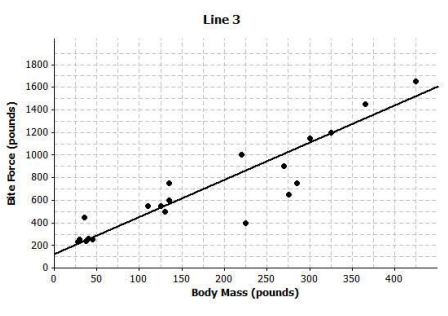
The scatter plots below show different lines that students used to model the relationship between body mass (in pounds) and bite force (in pounds) for crocodilians.
Match each graph to one of the equations below, and explain your reasoning. Let B represent bite force (in pounds) and W represent body mass (in pounds).
Equation 1
B = 3.28W + 126
Equation 2
B = 3.04W + 351
Equation 3
B = 2.16W + 267
Equation:
Answer:
Equation: 3
The intercept of 267 appears to match the graph, which has the second largest intercept.
Equation:
Answer:
Equation: 2
The intercept of Equation 2 is larger, so it matches Line 2, which has a y – intercept closer to 400.
Equation:
Answer:
Equation: 1
The intercept of Equation 1 is the smallest, which seems to match the graph.
b. Which of the lines would best fit the trend in the data? Explain your thinking.
Answer:
Answers will vary. Line 3 would be better than the other two lines. Line 1 is not a good fit for larger weights, and Line 2 is above nearly all of the points and pretty far away from most of them. It looks like Line 3 would be closer to most of the points.
Question 4.
Comment on the following statements:
a. A line modeling a trend in a scatter plot always goes through the origin.
Answer:
Some trend lines go through the origin, but others may not. Often, the value (0, 0) does not make sense for the data.
b. If the response variable increases as the independent variable decreases, the slope of a line modeling the trend is negative.
Answer:
If the trend is from the upper left to the lower right, the slope for the line is negative because for each unit increase in the independent variable, the response decreases.
Eureka Math Grade 8 Module 6 Lesson 9 Exit Ticket Answer Key
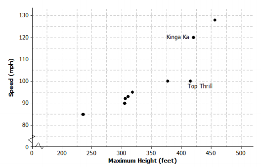
Question 1.
The scatter plot below shows the height and speed of some of the world’s fastest roller coasters. Draw a line that you think is a good fit for the data.
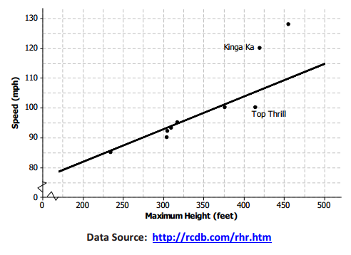
Answer:
Students would draw a line based on the goal of a best fit for the given scatter plot. A possible line is drawn below.
Question 2.
Find the equation of your line. Show your steps.
Answer:
Answers will vary based on the line drawn. Let S equal the speed of the roller coaster and H equal the maximum height of the roller coaster.
m = \(\frac{115 – 85}{500 – 225}\) ≈ 0.11
S = 0.11H + b
85 = 0.11(225) + b
b ≈ 60
Therefore, the equation of the line drawn in Problem 1 is S = 0.11H + 60.
Question 3.
For the two roller coasters identified in the scatter plot, use the line to find the approximate difference between the observed speeds and the predicted speeds.
Answer:
Answers will vary depending on the line drawn by a student or the equation of the line. For the Top Thrill, the maximum height is about 415 feet and the speed is about 100 miles per hour. The line indicated in Problem 2 predicts a speed of 106 miles per hour, so the difference is about 6 miles per hour over the actual speed. For the Kinga Ka, the maximum height is about 424 feet with a speed of 120 miles per hour. The line predicts a speed of about 107 miles per hour, for a difference of 13 miles per hour under the actual speed. (Students can use the graph or the equation to find the predicted speed.)