Engage NY Eureka Math Algebra 2 Module 4 Lesson 26 Answer Key
Eureka Math Algebra 2 Module 4 Lesson 26 Exercise Answer Key
Opening Exercise:
Previously, you considered the random assignment of 10 tomatoes into two distinct groups of 5 tomatoes, Group A and Group B. With each random assignment, you calculated Diiff = \(\overline{\boldsymbol{x}}_{A}\) – \(\overline{\boldsymbol{x}}_{B}\), the difference between the mean weight of the 5 tomatoes in Group A and the mean weight of the 5 tomatoes in Group B.
a. Summarize in writing what you learned in the last lesson. Share your thoughts with a neighbor.
Answer:
In the last lesson, when the single group of observations was randomly divided into two groups, the means of these two groups differed by chance. In some cases, the difference in the means of these two groups was very small (or 0), but in other cases, this difference was larger.
However, in order to determine which differences were typical and ordinary versus unusual and rare, a sense of the center, spread, and shape of the distribution of possible differences is needed.
b. Recall that 5 of these 10 tomatoes are from plants that received a nutrient treatment in the hope of growing bigger tomatoes. But what if the treatment was not effective? What difference would you expect to find between the group means?
Answer:
I would expect there to be no difference between the mean of Group A and the mean of Group B when performing these randomization assignments; in other words, I would expect a value of Diff equal to 0.
Exercises 1 – 2: The Distribution of Diff and Why 0 Is Important
In the previous lesson, 3 instances of tomato randomization were considered. Imagine that the random assignment was conducted an additional 247 times, and 250 Diff values were computed from these 250 random assignments. The results are shown graphically below in a dot plot where each dot represents the Diff value that results from a random assignment.
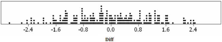
This dot plot will serve as your randomization distribution for the Diff statistic in this tomato randomization example. The dots are placed at increments of 0.04 ounces.
Exercise 1.
Given the distribution picture above, what is the approximate value of the median and mean of the distribution? Specifically, do you think this distribution is centered near a value that implies “No Difference” between Group A and Group B?
Answer:
The Diff value that implies “No Difference” between Group A and Group B would be 0. From visual inspection, the approximate value of the median and mean of the distribution appears to be near 0, based on the near symmetry and the center of the distribution. (Note: The actual mean, in this case, is -0.053 ounces, and the median is -0.08 ounces – both just slightly below 0.)
Exercise 2.
Given the distribution pictured above and based on the simulation results, determine the approximate probability of obtaining a Duff value in the cases described in (a), (b), and (c).
a. Of 1. 64 ounces or more
Answer:
17 out of 250 are 1.64 or more.
\(\frac{17}{250}\) = 0.068 = 6.8%
b. Of -0.80 ounces or less
Answer:
69 out of 250 are -0.80 or less.
\(\frac{69}{250}\) = 0.276 = 27.6%
c. Within 0.80 ounces of 0 ounces
Answer:
121 out of 250 are between -0.80 and 0.80.
\(\frac{121}{250}\) = 0.484 = 48.4%
d. How do you think these probabilities could be useful to people who are designing experiments?
Answer:
The probabilities could be used to help determine if the differences occurred by chance or not.
Exercises 3 – 5: Statistically Significant Diff Values
In the context of a randomization distribution that is based upon the assumption that there is no real difference between the groups, consider a Duff value of X to be statistically significant If there is a low probability of obtaining a result that is as extreme as or more extreme than X.
Exercise 3.
Using that definition and your work above, would you consider any of the Diff values below to be statistically significant? Explain.
a. 1.64 ounces
Answer:
Possibly statistically significant; an event with a 6.8% probability of occurring is not a very frequent occurrence.
b. -0.80 ounces
Answer:
Not statistically significant; an event with a 27.6% probability of occurring is a fairly common occurrence.
c. Values within 0.80 ounces of 0 ounces
Answer:
Values within 0.80 ounces of 0 ounces are not statistically significant; these values are not very far from 0, and they are fairly common. Also, given the symmetry, if -0.80 is not considered statistically significant (in part (b), above), then values that are closer to 0 would also not be considered statistically significant.
Exercise 4.
In the previous lessons, you obtained Diff values of 0.28 ounces, 2.44 ounces, and 0 ounces for 3 different tomato randomizations. Would you consider any of those values to be statistically significant for this distribution? Explain.
Answer:
The values of 0 and 0.28 ounces would not be statistically significant based on the work above and the fact that neither value is very far from 0 in the distribution. However, the value of 2.44 would be statistically significant because it is very far from 0 (maximum observation), and there is only a 1 in 250 chance (0.004, or 0.4% chance)
of obtaining a value that extreme in this distribution.
Exercise 5.
Recalling that Diff is the mean weight of the 5 Group A tomatoes minus the mean weight of the 5 Group B tomatoes, how would you explain the meaning of a Duff value of 1.64 ounces in this case?
Answer:
The 5 tomatoes of Group A have a mean weight that is 1.64 ounces higher than the mean weight of Group B’s 5 tomatoes.
Exercises 6 – 8: The Implication of Statistically Significant Diff Values
Keep in mind that for reasons mentioned earlier, the randomization distribution above is demonstrating what is likely to happen by chance alone if the treatment was not effective. As stated in the previous lesson, you can use this randomization distribution to assess whether or not the actual difference in means obtained from your experiment (the difference between the mean weight of the 5 actual control group tomatoes and the mean weight of the 5 actual treatment group tomatoes) is consistent with usual chance behavior. The logic is as follows:
→ If the observed difference is “extreme” and not typical of chance behavior, it may be considered statistically significant and possibly not the result of chance behavior.
→ If the difference is not the result of chance behavior, then maybe the difference did not just happen by chance alone.
→ If the difference did not just happen by chance alone, maybe the difference you observed is caused by the treatment in question, which, in this case, is the nutrient. In the context of our example, a statistically significant Diff value provides evidence that the nutrient treatment did in fact yield heavier tomatoes on average.
Exercise 6.
For reasons that will be explained in the next lesson, for your tomato example, Diff values that are positive and statistically significant will be considered as good evidence that your nutrient treatment did in fact yield heavier tomatoes on average.
Again, using the randomization distribution shown earlier in the lesson, which (if any) of the following Dill values would you consider to be statistically significant and lead you to think that the nutrient treatment did in fact yield heavier tomatoes on average? Explain for each case.
Diff= 0.4, Diff= 0.8, Diff= 1.2, Diff= 1.6, Diff= 2.0, Diff= 2.4
Answer:
Diff = 0.4: not statistically significant; not very far from 0; 91 of 250 values (36.4%) are greater than or equal to 0.4.
Diff = 0.8: not statistically significant; not very far from 0; 64 of 250 values (25.6%) are greater than or equal to 0.8
Diff = 1.2: not statistically significant; not too far from 0; 38 of 250 values (15.2%) are greater than or equal to 1.2.
Diff = 1.6: possibly statistically significant; somewhatfarfrom 0; 21 of 250 values (8.4%) are greater than or equal to 1.6.
Diff = 2.0: statistically significant; veryfarfrom 0; only 11 of 250 values (4.4%) are greater than or equal to 2.0.
Diff = 2.4: statistically significant; very far from 0; only 3 of 250 values (1.2%) are greater than or equal to 2.4.
Exercise 7.
In the first random assignment in the previous lesson, you obtained a Diff value of 0.28 ounce. Earlier in this lesson, you were asked to consider if this might be a statistically significant value. Given the distribution shown in this lesson, if you had obtained a Diff value of 0.28 ounces in your experiment and the 5 Group A tomatoes had been the “treatment” tomatoes that received the nutrient, would you say that the Diff value was extreme enough to support a conclusion that the nutrient treatment yielded heavier tomatoes on average? Or do you think such a Dill value may just occur by chance when the treatment is ineffective? Explain.
Answer:
I would say that the Duff value of 0. 28 was NOT extreme enough to support a conclusion that the nutrient treatment yielded heavier tomatoes on average. Such a Diff value may just occur by chance in this case. See earlier work in Exercise 4. Also, referencing the question above, 0.28 is even closer to 0 than other not statistically significant values.
Exercise 8.
In the second random assignment in the previous lesson, you obtained a Diff value of 2.44 ounces. Earlier In this lesson, you were asked to consider if this might be a statistically significant value. Given the distribution shown in this lesson, if you had obtained a Diff value of 2.44 ounces in your experiment and the 5 Group A tomatoes had been the “treatment” tomatoes that received the nutrient, would you say that the Diff value was extreme enough to support a conclusion that the nutrient treatment yielded heavier tomatoes on average? Or do you think such a Diff value may just occur by chance when the treatment is ineffective? Explain.
Answer:
I would say that the Diff value of 2.44 was extreme enough to support a conclusion that the nutrient treatment
yielded heavier tomatoes on average. This most likely did NOT just occur by chance. See earlier work in Exercise 4.
Also, referencing the question above, 2.44 is even farther away from 0 than other statistically significant values.
Eureka Math Algebra 2 Module 4 Lesson 26 Problem Set Answer Key
In each of the 3 cases below, calculate the Difivalue as directed, and write a sentence explaining what the Duff value means in context. Write the sentence for a general audience.
Question 1.
Group A: 8 dieters lost an average of 8 pounds, \(\overline{\boldsymbol{x}}_{A}\) = -8.
Group B: 8 nondieters lost an average of 2 pounds over the same time period, so \(\overline{\boldsymbol{x}}_{B}\) = -2.
Calculate and interpret Diff = \(\overline{\boldsymbol{x}}_{A}\) – \(\overline{\boldsymbol{x}}_{B}\).
Diff = \(\overline{\boldsymbol{x}}_{A}\) – \(\overline{\boldsymbol{x}}_{B}\)= -8 – (-2) = -6. The 8 dieters lost an average of 6 pounds more than the 8 nondieters.
Question 2.
Group A: 11 students were on average 0.4 seconds faster in their 100-meter run times after following a new training regimen.
Group B: 11 students were on average 0. 2 seconds slower in their 100-meter run times after not following any new training regimens.
Calculate and interpret Diff= \(\overline{\boldsymbol{x}}_{A}\) – \(\overline{\boldsymbol{x}}_{B}\).
Answer:
Diff = -0.4 – 0.2 = -0.6. The 11 students following the new training regimen were on average 0.6 seconds faster in their 100-meter run times than the 11 students not following any new training regimens.
Question 3.
Group A: 20 squash that have been grown in an irrigated field have an average weight of 1. 3 pounds.
Group B: 20 squash that have been grown In a nonirrigated field have an average weight of 1.2 pounds. Calculate and interpret Diff = \(\overline{\boldsymbol{x}}_{A}\) – \(\overline{\boldsymbol{x}}_{B}\)
Answer:
Diff = 1.3 – 1.2 = 0. 1. The 20 squash grown in an irrigated field have an average weight that is 0.1 pound higher than the 20 squash grown in a nonirrigated field.
Question 4.
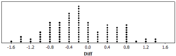
Using the randomization distribution shown below, what is the probability of obtaining a Diff value of -0. 6 or less?
Answer:
\(\frac{29}{100}\) = 0.29, which is 29%
Question 5.
Would a Diff value of -0. 6 or less be considered a statistically significant difference? Why or why not?
Answer:
No. -0.6 is not far from 0, and the probability of obtaining a Diff value of -0. 6 or less is 29%.
Question 6.
Using the randomization distribution shown in Problem 4, what is the probability of obtaining a Diff value of -1. 2 or less?
Answer:
The probability of obtaining a Diff value of -1.2 or less is 6 out of 100, or 6%.
Question 7.
Would a Diff value of -1.2 or less be considered a statistically significant difference? Why or why not?
Possibly statistically significant. -1.2 is far from 0, and the probability of obtaining a Diff value of -1.2 or less is only 6%. The value provides evidence that the new treatment may be effective in relieving pain.
Eureka Math Algebra 2 Module 4 Lesson 26 Exit Ticket Answer Key
Medical patients who are in physical pain are often asked to communicate their level of pain on a scale of 0 to 10 where 0 means no pain and 10 means worst pain. (Note: Sometimes a visual device with pain faces is used to accommodate the reporting of the pain score.) Due to the structure of the scale, a patient would desire a lower value on this scale after treatment for pain.
Imagine that 20 subjects participate in a clinical experiment and that a variable of “ChangeinScore” is recorded for each subject as the subject’s pain score after treatment minus the subject’s pain score before treatment. Since the expectation is that the treatment would lower a patient’s pain score, you would desire a negative value for “ChangeinScore.” For example, a “ChangeinScore” value of -2 would mean that the patient was in less pain (for example, now at a 6, formerly at an 8).
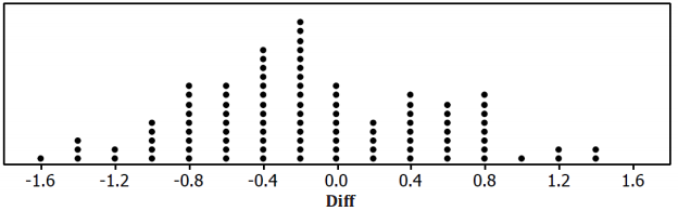
Recall that Diff = \(\overline{\boldsymbol{x}}_{A}\) – \(\overline{\boldsymbol{x}}_{B}\). Although the 20 “ChangeinScore” values for the 20 patients are not shown here, below is a randomization distribution of the value Duff based on 100 random assignments of these 20 observations into two groups of 10 (Group A and Group B).
Question 1.
From the distribution above, what is the probability of obtaining a Diff value of -1 or less?
Answer:
\(\frac{11}{100}\) = 0.11, which is 11%
Question 2.
With regard to this distribution, would you consider a Diff value of -.4 to be statistically significant? Explain.
Answer:
No. The value is not far from 0, and 42 of the 100 values in the distribution are at or below -0.4.
Question 3.
a. With regard to how Diff I calculated if Group A represented a group of patients in your experiment who received a new pain relief treatment and Group B received a pill with no medicine (called a placebo), how would you interpret a Diff value of -1.4 pain scale units in context?
Answer:
The group that received the pain relief treatment had an average reduction in pain that was 1.4 units better (lower) than the group that received the placebo.
b. Given the distribution above, if you obtained Diff value such as -1.4 from your experiment, would you consider that to be significant evidence of the new treatment being effective on average in relieving pain? Explain.
Answer:
Yes. -1.4 is far from 0, and the probability of obtaining a Diff value of -1.4 or less is only 4%. The value provides evidence that the new treatment may be effective in relieving pain.