Engage NY Eureka Math Algebra 2 Module 4 Lesson 17 Answer Key
Eureka Math Algebra 2 Module 4 Lesson 17 Exercise Answer Key
Exercises 1 – 6: Standard Deviation for Proportions
In the previous lesson, you used simulated sampling distributions to learn about sampling variability in the sample proportion and the margin of error when using a random sample to estimate a population proportion. However, finding a margin of error using simulation can be cumbersome and can take a long time for each situation.
Fortunately, given the consistent behavior of the sampling distribution of the sample proportion for random samples, statisticians have developed a formula that will allow you to find the margin of error quickly and without simulation.
Exercise 1.
30% of students participating in sports at Union High School are female (a proportion of 0.30).
a. If you took many random samples of 50 students who play sports and made a dot plot of the proportion of female students in each sample, where do you think this distribution will be centered? Explain your thinking.
Answer:
Answers will vary. Since 30% of 50 is 15, I would expect the sampling distribution to be centered around female students.
b. In general, for any sample size, where do you think the center of a simulated distribution of the sample proportion of female students in sports at Union High School will be?
Answer:
The sampling distribution should be centered at around 0.3. Some samples will result in a sample proportion of female students that is greater than 0.3, and some will result in a sample proportion of female students that is less than 0.3, but the sample proportions should center around 0.3.
Exercise 2.
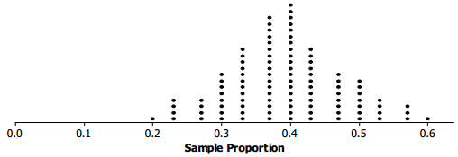
Below are two simulated sampling distributions for the sample proportion of female students in random samples from all the students at Union High School.
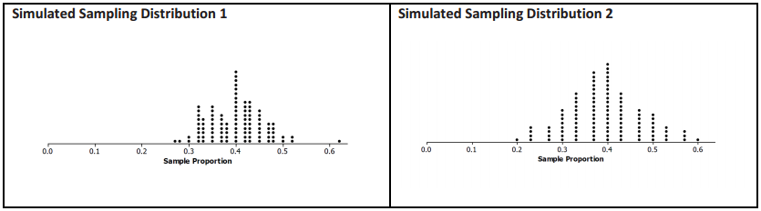
a. Based on the two sampling distributions above, what do you think is the population proportion of female students?
Answer:
Answers will vary, but students should give an answer around 0.4.
b. One of the sampling distributions above is based on random samples of size 30, and the other is based on random samples of size 60. Which sampling distribution corresponds to the sample size of 30? Explain your choice.
Answer:
Simulated Sampling Distribution 2 corresponds to the sample size of 30. I chose this one because it is more spread out – there is more sample-to-sample variability in Simulated Sampling Distribution 2 than in Simulated Sampling Distribution 1.
Exercise 3.
Remember from your earlier work in statistics that distributions were described using shape, center, and spread. How was spread measured?
Answer:
The spread of distribution was measured with either the standard deviation or (sometimes) the interquartile range.
Exercise 4.
For random samples of size n, the standard deviation of the sampling distribution of the sample proportion can be calculated using the following formula:
standard deviation = \(\sqrt{\frac{p(1-p)}{n}}\),
where p is the value of the population proportion and n is the sample size.
a. If the proportion of female students at Union High School Is 0.4, what is the standard deviation of the distribution of the sample proportions of female students for random samples of size 50? Round your answer to three decimal places.
Answer:
\(\sqrt{\frac{(0.4)(0.6)}{50}}\) ≈ 0.069
b. The proportion of males at Union High School is 0. 6. What is the standard deviation of the distribution of the sample proportions of male students for random samples of size 50? Round your answer to three decimal places.
Answer:
\(\sqrt{\frac{(0.6)(0.4)}{50}}\) ≈ 0.069
c. Think about the graphs of the two distributions in parts (a) and (b). Explain the relationship between your answers using the center and the spread of the distributions.
Answer:
The two distributions are alike, but one is centered at 0.6 and the other at 0.4. The spread, as measured by the standard deviation of the two distributions, will be the same.
Exercise 5.
Think about the simulations that your class performed in the previous lesson and the simulations in Exercise above.
a. Was the sampling variability in the sample proportion greater for samples of size 30 or for samples of size 50? In other words, does the sample proportion tend to vary more from one random sample to another when the sample size is 30 or 50?
Answer:
There was more variability from sample to sample when the sample size was 30.
b. Explain how the observation that the variability in the sample proportions decreases as the sample size increases is supported by the formula for the standard deviation of the sample proportion.
Answer:
You divide by n in the formula, and as n (o positive whole number) increases, the result of the division will be smaller.
Exercise 6.
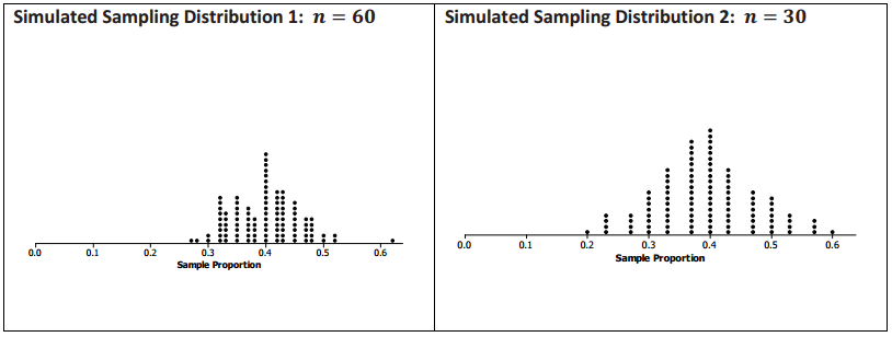
Consider the two simulated sampling distributions of the proportion of female students in Exercise 2 where the population proportion was 0.4. Recall that you found n = 60 for Distribution 1 and n = 30 for Distribution 2.
a. Find the standard deviation for each distribution. Round your answer to three decimal places.
Answer:
In Simulated Sampling Distribution 1, n = 60, and the standard deviation is 0.063.
In Simulated Sampling Distribution 2, n = 30, and the standard deviation is 0.089.
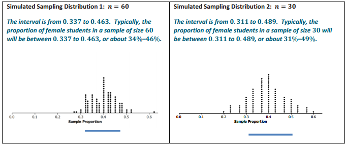
b.
Make a sketch, and mark off the intervals one standard deviation from the mean for each of the two distributions. Interpret the intervals in terms of the proportion of female students in a sample.
Answer:
In general, three results about the sampling distribution of the sample proportion are known.
→ The sampling distribution of the sample proportion is centered at the actual value of the population proportion, p.
→ The sampling distribution of the sample proportion is less variable for larger samples than for smaller samples.
→ The variability in the sampling distribution is described by the standard deviation of the distribution, and the standard deviation of the sampling distribution for random samples of size n is \(\sqrt{\frac{p(1-p)}{n}}\), where p is the value of the population proportion.
This standard deviation is usually estimated using the sample proportion, which is denoted by (read as p-hat), to distinguish it from the population proportion. The formula for the estimated standard deviation of the distribution of sample proportions is \(\sqrt{\frac{p(1-p)}{n}}\).
→ As long as the sample size is large enough that the sample includes at least 10 successes and failures, the sampling distribution is approximately normal in shape. That is, a normal distribution would be a reasonable model for the sampling distribution.
Exercises 7 – 12: Using the Standard Deviation with Margin of Error
Exercise 7.
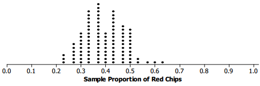
In the work above, you investigated a simulated sampling distribution of the proportion of female students in a sample of size 30 drawn from a population with a known proportion of 0.4 female students. The simulated distribution of the proportion of red chips in a sample of size 30 drawn from a population with a known proportion of 0.4 is displayed below.
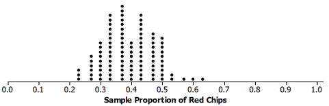
a. Use the formula for the standard deviation of the sample proportion to calculate the standard deviation of the sampling distribution. Round your answer to three decimal places.
Answer:
The standard deviation should be about 0.089.
b. The distribution from Exercise 2 for a sample of size 30 is below. How do the two distributions compare?
Answer:
The shapes of the two sampling distributions of the proportions are slightly different, but they both center at 0.4 and have the same estimated standard deviation, 0.089.
c. How many of the values of the sample proportions are within one standard deviation of 0.4? How many are within two standard deviations of 0.4?
Answer:
The typical distance of the values from 0.4 is one standard deviation, between 0.311 and 0.489. All but two of the values are within two standard deviations from 0.4, or between 0.222 and 0. 578. See the dot plot below.
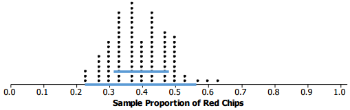
In general, for a known population proportion, about 95% of the outcomes of a simulated sampling distribution of a sample proportion will fall within two standard deviations of the population proportion. One caution is that If the proportion is close to 1 or 0, this general rule may not hold unless the sample size is very large.
You can build from this to estimate a proportion of successes for an unknown population proportion and calculate a margin of error without having to carry out a simulation.
If the sample is large enough to have at least 10 of each of the two possible outcomes in the sample but small enough to be no more than 10% of the population, the following formula (based on an observed sample proportion) can be used to calculate the margin of error.
The standard deviation involves the parameter p that is being estimated. Because p is often not known, statisticians replace p with its estimate fi in the standard deviation formula. This estimated standard deviation is called the standard error of the sample proportion.
Exercise 8.
a. Suppose you draw a random sample of 36 chips from a mystery bag and find 20 red chips. Find, the sample proportion of red chips, and the standard error.
Answer:
\(\widehat{\boldsymbol{p}}\) = \(\frac{20}{36}\) ≈ 0.56, and the standard error is \(\sqrt{\frac{\hat{p}(1-\hat{p})}{n}}=\sqrt{\frac{(0.56)(0.44)}{36}}\) ≈ 0.083.
b. Interpret the standard error.
Answer:
The sample proportion was 0.56, so I estimate that the proportion of red chips in the bag is 0.56. The actual population proportion probably isn’t exactly equal to 0.56, but I expect that my estimate is within 0.083 of the actual value.
When estimating a population proportion, margin of error can be defined as the maximum expected difference between the value of the population proportion and a sample estimate of that proportion (the farthest away from the actual population value that you think your estimate is likely to be).
If \(\widehat{\boldsymbol{p}}\) is the sample proportion for a random sample of size n from some population and if the sample size is large enough,
estimated margin of error = 2\(\sqrt{\frac{\bar{p}(1-\bar{p})}{n}}\).
Exercise 9.
Henri and Terence drew samples of size 50 from a mystery bag. Henri drew 42 red chips, and Terence drew 40 red chips. Find the margins of error for each student.
Answer:
Henri’s estimated margin of error is 0.104; Terence’s estimated margin of error is 0.113.
Exercise 10.
Divide the problems below among your group, and find the sample proportion of successes and the estimated margin of error in each situation:
a. Sample of size 20, 5 red chips
Answer:
Sample proportion of red chips is 0.25, which is 25%; estimated margin of error is 0.194, which is 19.4%.
b. Sample of size 40, 10 red chips
Answer:
Sample proportion of red chips is 0.25, which is 25%; estimated margin of error is 0. 137, which is 13.7%.
c. Sample of size 80, 20 red chips
Answer:
Sample proportion of red chips is 0.25, which is 25%; estimated margin of error is 0.097, which is 9.7%.
d. Sample of size 100, 25 red chips
Answer:
Sample proportion of red chips is 0.25, which is 25%; estimated margin of error is 0.087, which is 8.7%.
Exercise 11.
Look at your answers to Exercise 2.
a. What conjecture can you make about the relation between sample size and margin of error? Explain why your conjecture makes sense.
Answer:
As the sample size increases, the margin of error decreases. 1f you have a larger sample size, you can get a better estimate of the proportion of successes that are in the population, so the margin of error should be smaller.
b. Think about the formula for a margin of error. How does this support or refute your conjecture?
Answer:
In the formula for the margin of error, the sample size is in the denominator of a fraction. if the sample size is large, that means the result of the division gets smaller. So, if the proportion is the same for three different-sized random samples, the smallest result would be when you divided by the largest sample size.
Exercise 12.
Suppose that a random sample of size loo will be used to estimate a population proportion.
a. Would the estimated margin of error be greater if \(\widehat{\boldsymbol{p}}\) = 0.4 or \(\widehat{\boldsymbol{p}}\) = 0.5? Support your answer with appropriate calculations.
Answer:
For P̂ = 0.4: estimated margin of error = 2\(\sqrt{\frac{(0.4)(0.6)}{100}}\) ≈ 0.098
For \(\widehat{\boldsymbol{p}}\) = 0.5: estimated margin of error = 2\(\sqrt{\frac{(0.5)(0.5)}{100}}\) ≈ 0.100
The estimated margin of error is greater when \(\widehat{\boldsymbol{p}}\) = 0.5.
b. Would the estimated margin of error be greater if = 0.5 or ji = 0.8? Support your answer with appropriate calculations.
Answer:
For p̂ = 0.5; estimated margin of error = 2\(\sqrt{\frac{(0.5)(0.5)}{100}}\) ≈ 0.100
For p̂ = 0.8; estimated margin of error = 2\(\sqrt{\frac{(0.8)(0.2)}{100}}\) ≈ 0.080
The estimated margin of error is greater when p̂ = 0. 5.
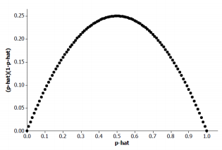
c.
For what value of do you think the estimated margin of error will be greatest? (Hint: Draw a graph of p̂(1 – p̂ ) as p̂ ranges from 0 to 1.)
Answer:
The estimated margin of error is greater when p̂ = 0.5. The value of p̂(1 – p̂) is greatest when p̂ = 0.5. (See graph below.) This value is in the numerator of the fraction in the formula for the margin of error, so the margin of error is greatest when p̂ = 0.5.
Eureka Math Algebra 2 Module 4 Lesson 17 Problem Set Answer Key
Question 1.
Different students drew random samples of size 50 from the mystery bag. The number of red chips each drew is given below. In each case, find the margin of error for the proportions of the red chips in the mystery bag.
a. 10 red chips
Answer:
The margin of error will be approximately 0.113.
b. 28 red chips
Answer:
The margin of error will be approximately 0.140.
c. 40 red chips
Answer:
The margin of error will be approximately 0.113.
Question 2.
The school newspaper at a large high school reported that 120 out of 200 randomly selected students favor assigned parking spaces. Compute the margin of error. Interpret the resulting interval in context.
Answer:
The margin of error will be 2\(\sqrt{\frac{(0.4)(0.6)}{200}}\). which is approximately 0.069. The resulting interval is 0.6 ± 0.069, or from 0,531 to 0.669. The proportion of students who favor assigned parking spaces is from 0.531 to 0.669.
Question 3.
A newspaper in a large city asked 500 women the following: “Do you use organic food products (such as milk, meats, vegetables, etc.)?” 280 women answered “yes.” Compute the margin of error, Interpret the resulting interval in context.
Answer:
The margin of error will be 2\(\sqrt{\frac{(0.56)(0.44)}{500}}\). which is approximately 0.044. The resulting interval is 0.56 ± 0.044 or from 0.516 to 0.604. The proportion of women who use organic food products is between 0.516 and 0.604.
Question 4.
The results of testing a new drug on 1,000 people with a certain disease found that 510 of them improved when they used the drug. Assume these 1,000 people can be regarded as a random sample from the population of all people with this disease. Based on these results, would it be reasonable to think that more than half of the people with this disease would improve if they used the new drug? Why or why not?
Answer:
The margin of error would be about 0.032, which is about 3.2%, which means that the sample proportion of 0.510 is likely to be within 0.032 of the value of the actual population proportion. That means that the population proportion might be as small as 0.478, which is 47.8%. So, it is not reasonable to think that more than half of the people with the disease would improve if they used the new drug.
Question 5.
A newspaper in New York took a random sample of 500 registered voters from New York City and found that 300 favored a certain candidate for governor of the state. A second newspaper polled 1,000 registered voters in upstate New York and found that 550 people favored this candidate. Explain how you would interpret the results.
Answer:
In New York City, the proportion of people who favor the candidate is 0.60 ± 0.044, which is the range from 0.556 to 0.644. In upstate New York, the proportion of people who favor this candidate is 0. 55 ± 0.031, which is the range from 0. 519 to 0.581.
Because the margins of error for the two candidates produce intervals that overlap, you cannot really soy that the proportion of people who prefer this candidate is different for people in New York City and people in upstate New York.
Question 6.
In a random sample of 1,500 students in a large suburban school, 1, 125 reported having a pet, resulting in the interval 0.75 ± 0. 022. In a large urban school, 840 out of 1,200 students reported having a pet, resulting in the interval 0.7 ± 0.026. Because these two intervals do not overlap, there appears to be a difference in the proportion of suburban students owning a pet and the proportion of urban students owning a pet.
Suppose the sample size of the suburban school was only 500, but 75% still reported having a pet. Also, suppose the sample size of the urban school was 600, and 70% still reported having a pet. Is there still a difference in the proportion of students owning a pet in suburban schools and urban schools? Why does this occur?
Answer:
The resulting intervals are as follows:
For suburban students: 0.75 ± 2\(\sqrt{\frac{0.75(0.25)}{500}}\) ≈ 0.75 ± 0.039, or from 0.711 to 0.789.
For urban students: 0.7 ± 2\(\sqrt{\frac{0.7(0.3)}{600}}\) ≈ 0.7 ± 0.037, or from 0.663 to 0.737.
No, there does not appear to be a difference in the proportion of students owning a pet in suburban and urban schools. This occurred because the margins of error are larger due to the smaller sample size.
Question 7.
Find an article in the media that uses a margin of error. Describe the situation (an experiment, an observational study, a survey), and interpret the margin of error for the context.
Answer:
Students might bring in poll results from a newspaper.
Eureka Math Algebra 2 Module 4 Lesson 17 Exit Ticket Answer Key
Question 1.
Find the estimated margin of error when estimating the proportion of red chips in a mystery bag if 18 red chips were drawn from the bag in a random sample of 50 chips.
Answer:
The margin of error would be 0. 136.
Question 2.
Explain what your answer to Problem 1 tells you about the number of red chips in the mystery bag.
Answer:
The sample proportion of 0.36 is likely to be within 0. 136 of the actual value of the population proportion. This means that the proportion of red chips in the bag might be somewhere between 0.22 and 0.496, or about 22% – 50% red chips.
Question 3.
How could you decrease your margin of error? Explain why this works.
Answer:
The margin of error could be decreased by increasing sample size. The larger the sample size, the smaller the standard deviation, thus the smaller the margin of error.